Tuberculosis Detection in X-Rays With GUI Controls
by niammohseni in Workshop > Science
2227 Views, 4 Favorites, 0 Comments
Tuberculosis Detection in X-Rays With GUI Controls
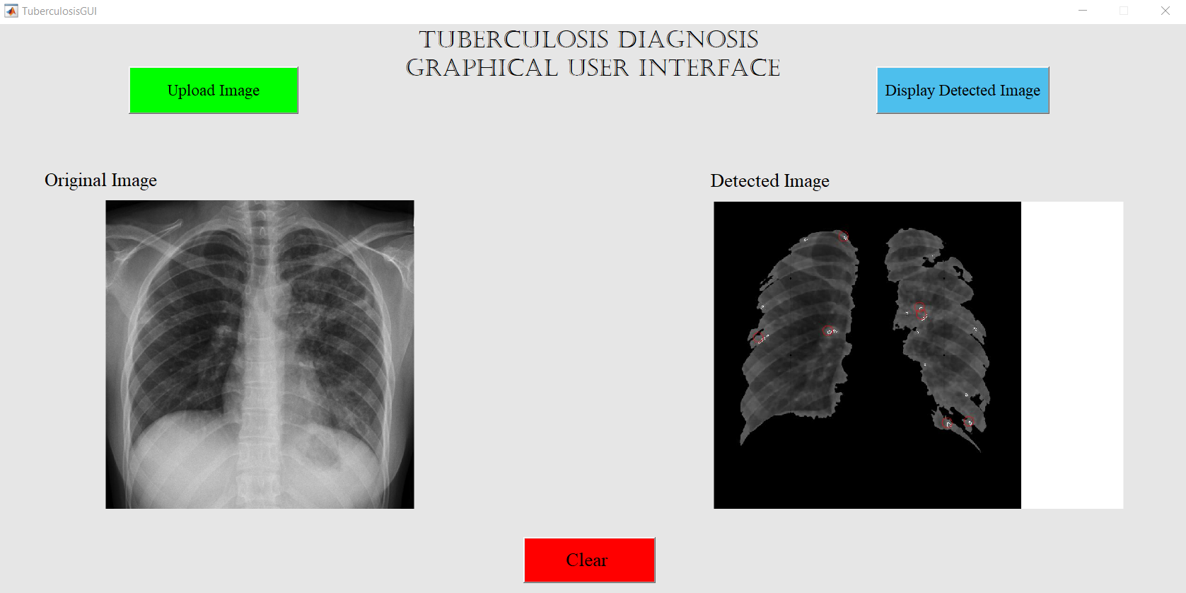
This code was designed entirely in MATLAB for the sole purpose of detecting regions of tuberculosis in x-rays of the disease. This program that we created is set up to work with a picture of a x-ray of the .png or .jpg file type, but this can be definitely be changed in the code to accept more file types. We wanted to make sure accurate results were gathered, so we implemented different techniques to ensure the best results in the time frame we had to work on this project.
The steps that we outline below will first begin with with the lung segmentation code that we will eventually turn into a function. The instructions will then proceed into the actual filtering and locating techniques that is the majority of the code. These include processes, like median filters, edge detection, image splitting, thresholds, and more! Then we will talk about creating the GUI itself with GUIDE, an app creator built into MATLAB. Finally, we will explain how we combined our code into the GUI to have a fully functional program.
Hopefully our instructions are clear and helpful to anyone reading. Any files that was used in the final product will be attached for download.
Getting Accurate X-Rays of Tuberculosis
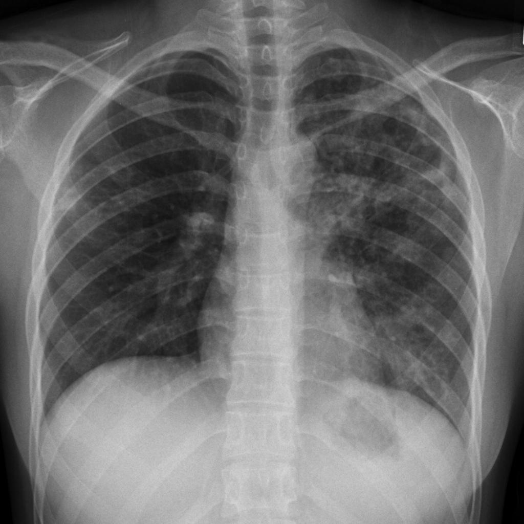
The funny thing is this was actually one of the hardest steps! Many of the images on google or other sites were either very low quality or just have watermarks plastered over the image. The trick to finding a great image is that if you are looking on google, make sure to set search filtering to large images. This change will ensure only high resolution images will be present in your search. Or you can just use a trusted image database that contain such images like: https://ceb.nlm.nih.gov/repositories/tuberculosis-chest-x-ray-image-data-sets/. This database has over 1.30 gigabytes of x-ray images, perfect for your use!
Creating a Simple File Grabber
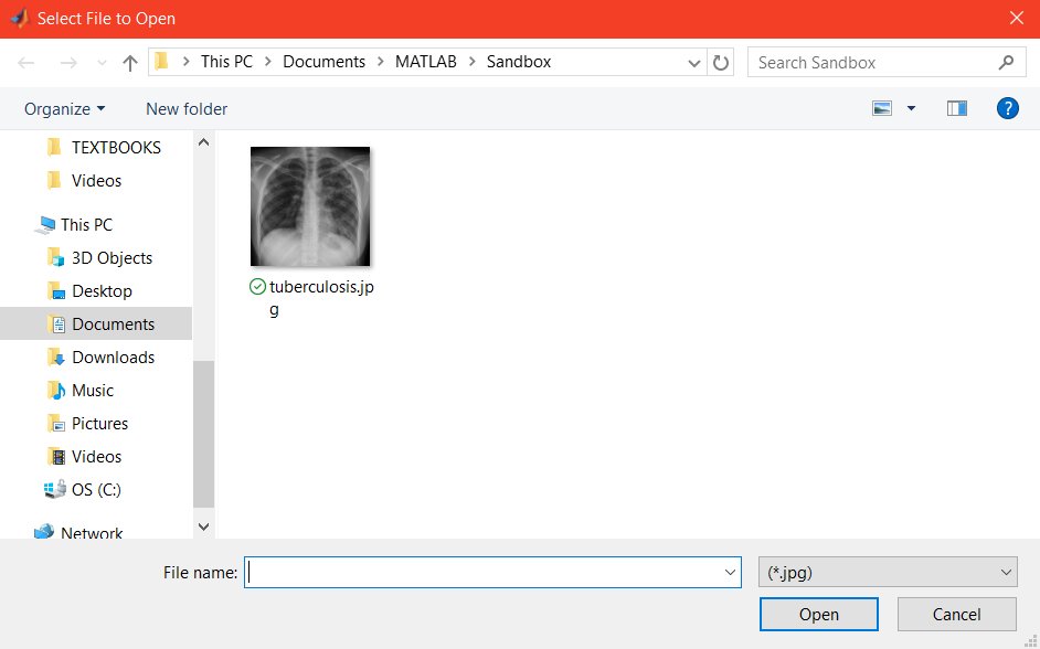

You have a file now on your computer, but that is useless if you do not even load it into MATLAB! We thought the best way of doing this was to have the user able to select the exact file through a menu that opens up. We also wanted to make sure that if the user cancels that there will not be an error message. All of this can be done, along with extra messages helping the user, using the code below:
-----------------------------------------------------------------------------------------------
waitfor(msgbox({'Please select the x-ray file.'})); % Have user understand to select a x-ray file before continuing
[file, folder] = uigetfile({'*.jpg';'*.png'}); % Allows users to select a file that is either a jpg or png
if isequal(file,0) % If the user cancels out the command window will display canceled
disp('Canceled');
return;
end Dir = [folder file]; % Creates an array of the folder location and the file name
-----------------------------------------------------------------------------------------------
The user has now selected the file he or she wants to user, but how do we put this file into our workspace? That’s easy! We simply use the Dir variable we created to load the file into MATLAB. The code will be:
grayImage = imread(Dir); % Reads the selected file from the folder with Dir
Segmenting the Lungs From the Image
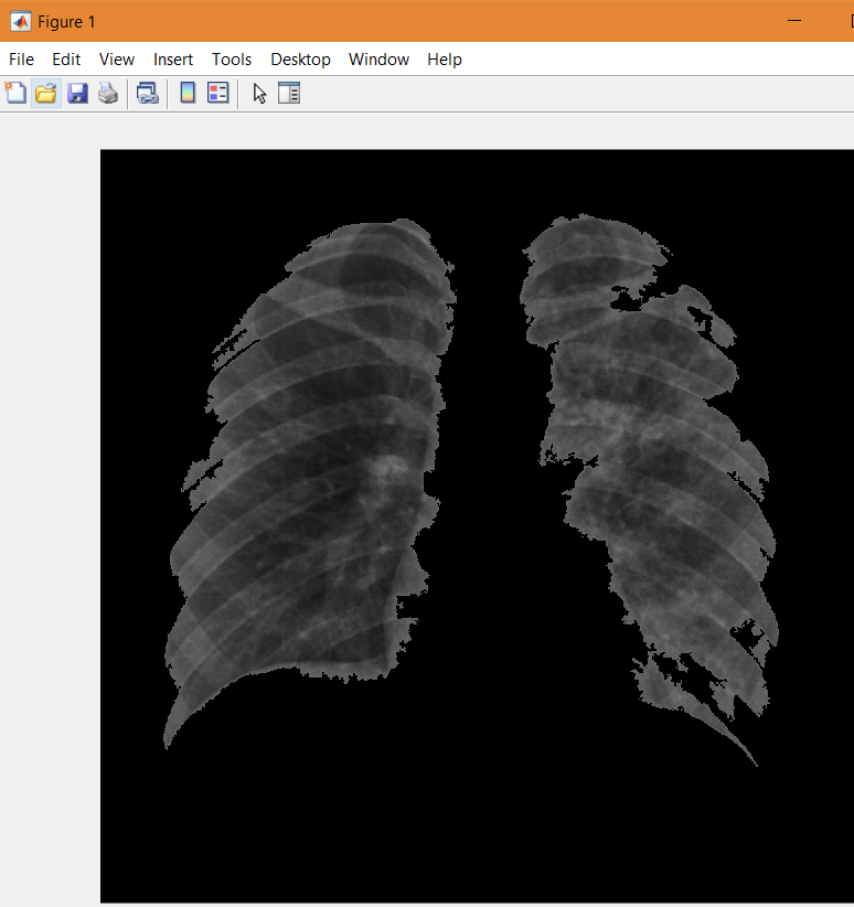
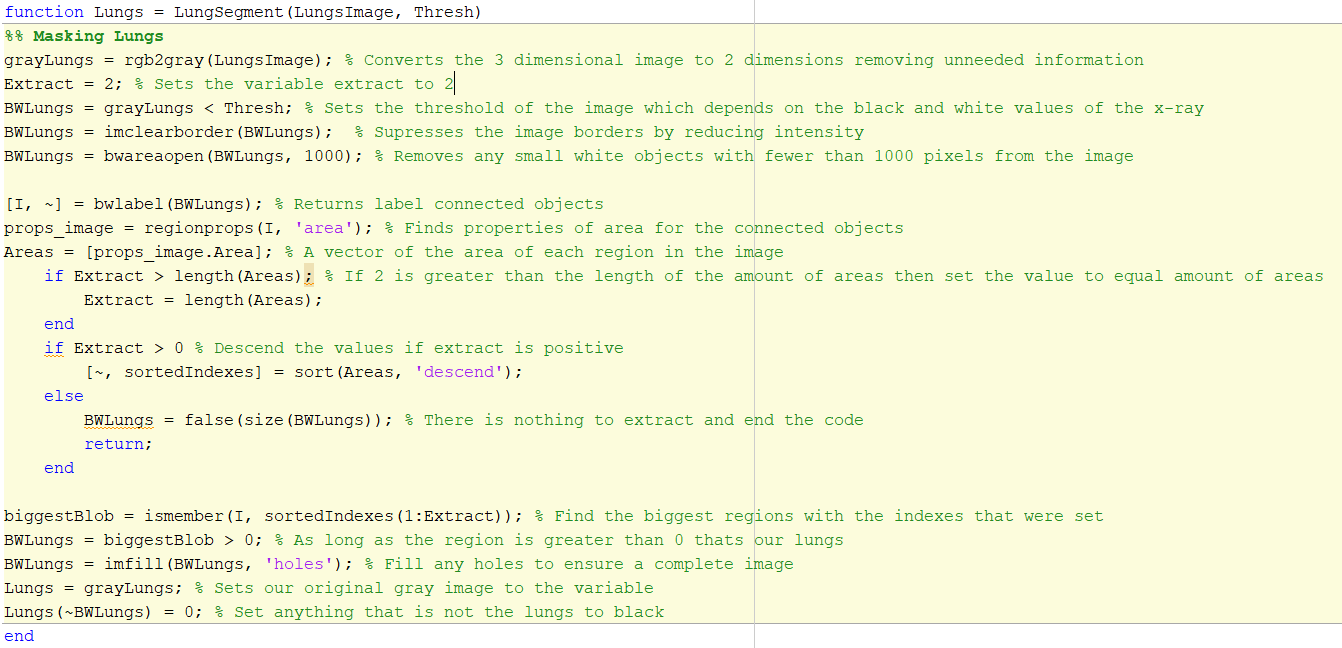
A big problem with detecting tuberculosis in x-ray images is all the useless extra information in the images, which includes the diaphragm, bones, trachea, and other regions. These unneeded regions would just make the extraction of the tuberculosis much more difficult and so we decided to simply pull out the lung regions. We did this through pulling out the biggest “blobs” in the image and masking it so we can pull it out of the original image.
By indicating the amount of regions we wanted to extract, two, and finding the areas that fit the lungs we can detect the regions once the correct threshold was set. The threshold for this image was best at a value of 100. The regions were then used with the gray image to make anything that was not the lung areas be black, so what is left is just the masked lungs from the gray image. We simply based The code below is used along with the UI file grabber as stated above:
grayLungs = rgb2gray(grayImage); % Converts the 3 dimensional image to 2 dimensions removing unneeded information
Extract = 2; % Sets the variable extract to 2
BWLungs = grayLungs < 100; % Sets the threshold of the image which depends on the black and white values of the x-ray
BWLungs = imclearborder(BWLungs); % Supresses the image borders by reducing intensity
BWLungs = bwareaopen(BWLungs, 1000); % Removes any small white objects with fewer than 1000 pixels from the image
[I, ~] = bwlabel(BWLungs); % Returns label connected objects
props_image = regionprops(I, 'area'); % Finds properties of area for the connected objects
Areas = [props_image.Area]; % A vector of the area of each region in the image
if Extract > length(Areas); % If 2 is greater than the length of the amount of areas then set the value to equal amount of areas
Extract = length(Areas);
end
if Extract > 0 % Descend the values if extract is positive
[~, sortedIndexes] = sort(Areas, 'descend');
else BWLungs = false(size(BWLungs)); % There is nothing to extract and end the code
return;
end
biggestBlob = ismember(I, sortedIndexes(1:Extract)); % Find the biggest regions with the indexes that were set
BWLungs = biggestBlob > 0; % As long as the region is greater than 0 that's our lungs
BWLungs = imfill(BWLungs, 'holes'); % Fill any holes to ensure a complete image
Lungs = grayLungs; % Sets our original gray image to the variable
Lungs(~BWLungs) = 0; % Set anything that is not the lungs to black
-----------------------------------------------------------------------------------------------
However, the problem with this code is that the threshold is a constant value and will not work for other images as well as the code being pretty large! We decided to turn the code into a function so one line of code can be used to segment the lungs. Instead of the variable grayImage and the value of 100, we put two put input values of LungsImage and Thresh. This is showcased in the image of this section.
Using a Message Box to Change Threshold Values and Running Lung Segmentation
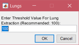
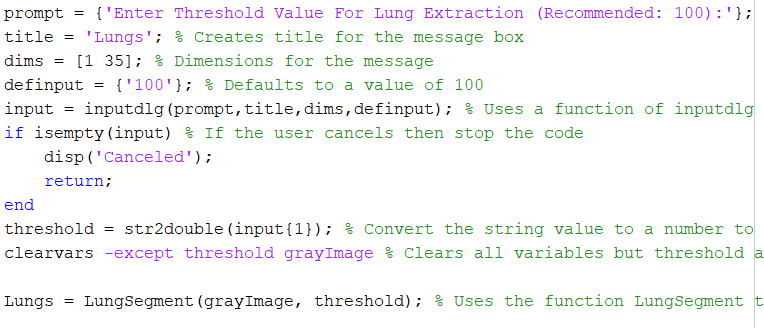
Since we changed the lung segmentation code to a function, we also want to give the user an option to set their own threshold. We did not want to use the input function as that would result in the use of the command window, which we are trying to eventually move past and just use a GUI. So, the next best option was to use the function inputdlg, which creates a message box.
All the message box had to do was ask the user set the value for the threshold and the code would run. If the threshold was too high or too low, then the user would be able to change it every time they run the code. We set 100 as the default threshold value as it worked well for the majority of our images. The code below creates a message box that the user can change the values of:
prompt = {'Enter Threshold Value For Lung Extraction (Recommended: 100):'}; % Tells the user what the meaning behind the value is
title = 'Lungs'; % Creates title for the message box
dims = [1 35]; % Dimensions for the message
definput = {'100'}; % Defaults to a value of 100
input = inputdlg(prompt,title,dims,definput); % Uses a function of inputdlg to allow the message box to appear and give the user access to edit the value
if isempty(input) % If the user cancels then stop the code
disp('Canceled');
return;
end
-----------------------------------------------------------------------------------------------
The code of course gives you an option for the user to cancel without causing an error in the command window. The issue with this code is that the value results in a cell. This can be fixed by simply converting the string to a numeric value with str2double:
threshold = str2double(input{1}); % Convert the string value to a number to use as a variable later in the code
clearvars -except threshold grayImage % Clears all variables but threshold and grayImage
Lungs = LungSegment(grayImage, threshold); % Uses the function LungSegment to pull out the lungs from the image
-----------------------------------------------------------------------------------------------
Just to keep our workspace clean, we deleted all variables except our image and our threshold which are all we need to run the function we created in the last step.
Resizing, Splitting the Image Up, and Detecting Regions of Interest
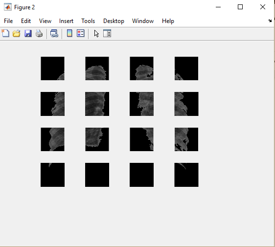
Resizing our image is a very simple, one line of code step. Our image has already been converted and therefore is simply an n x m matrix. An RGB image, however, is an n x m x 3 matrix and requires a little bit more thought to resize the image. Here we take our grayscale image and apply our image resize function already coded into MatLab. imresize is used to scale our image to the favorable n x m sizing we want to use, which in our case was a 720 x 720 pixel image.
GrayscaleImage = imresize(Lungs,[720 720]); % Resizes the image to 720x720 to ensure all images can be segmented
-----------------------------------------------------------------------------------------------
The first bit of information that goes within the imresize() function is our image that we have a desire to resize, after that we take a matrix bracket setup [] and implement our n and m lengths for the matrix e.g. [n m] where n is your rows and m is your columns. All together it should form a command statement like so,
Variable = imresize(desired_image, [n m]);
-----------------------------------------------------------------------------------------------
After resizing the image to a 720 x 720 pixel image, the more difficult step is to separate the image into 16 equal smaller images. The image is split into smaller images for the filtering and tuberculosis detection. With a separation of the image, our regions of interest are redefined and chosen more accurately than they would be if the image was defined as a whole. The size function is used, and we define three variables; rows, columns and the number of color bands our image contains. Two constants are important for the grayscale images, rows and columns. The number of color bands will always be one for our grayscaled images. Since we resized our image, rows and columns constants will always be equal to 720.
[rows, columns, numberOfColorBands] = size(GrayscaleImage); % Takes the size of the GrayScaleImage
-----------------------------------------------------------------------------------------------
In order to achieve this, we must first define a block size for our image, this is where the image resizing becomes quite useful. Now that we always have a definite size for our tuberculosis images, we can have a constant size for our smaller split images. We decided that sixteen smaller regions were a good amount to achieve accurate results in a timely manner. In order to get sixteen smaller regions, we need to create a 4 x 4 matrix of smaller images. In order to achieve this, we must divide our 720 x 720 image by 4, giving us a block size of 180 x 180. We define two variables, our block size rows as blockSizeR and blockSizeC for our block size columns. Both are set to 180.
blockSizeR = 180; % Rows in block block
SizeC = 180; % Columns in block
-----------------------------------------------------------------------------------------------
In order to get our block rows, which will always be 4, but for the purpose of good code practice we still calculate it here, we take the floor function which rounds our values to the smallest integer. We take the floor function and apply it to our rows divided by our block size constants.
wholeBlockRows = floor(rows / blockSizeR);
-----------------------------------------------------------------------------------------------
We then create a vector for our block rows, blockVectorR, by multiplying the values by a vector column of ones.
blockVectorR = [blockSizeR * ones(1, wholeBlockRows), rem(rows, blockSizeR)];
-----------------------------------------------------------------------------------------------
We repeat these two steps but with our column variables to get our column blocks.
wholeBlockCols = floor(columns / blockSizeC); blockVectorC = [blockSizeC * ones(1, wholeBlockCols), rem(columns, blockSizeC)];
-----------------------------------------------------------------------------------------------
Using an if-else statement we determine if our color bands are representative of a grayscale image or an RGB image. In our case, all the images will be grayscale, but we use the if-else statement as a backup measure in case this is not our case. We then create a cell array, using mat2cell which takes a matrix and makes it a cell. We input our grayscale image, and the row and column vector we just created.
if numberOfColorBands > 1 % Checks if the image is still in color
% If a color image also use numberOfColorBands
ca = mat2cell(GrayscaleImage, blockVectorR, blockVectorC, numberOfColorBands);
else % Grayscaled (all of our images)
ca = mat2cell(GrayscaleImage, blockVectorR, blockVectorC);
end
-----------------------------------------------------------------------------------------------
Using a nested for loop, we take a for loop that has an iteration length of our number of rows. The nested for loop runs for an iteration length of our number of columns. Every single iteration of the nested for loop subplots the column number plot, row and plot index which starts at 1 and increases by 1 with each run. We then take our cell array and plot the row and column with each loop. With each run we fill in the preallocated cell array with the values of each individual smaller image. By the end of the for loops, the cell array is our original image separated into sixteen smaller matrices.
for r = 1:numPlotsR % Run for the amount of rows there are
for c = 1:numPlotsC % Run for the amount of columns there are
% Specify the location for display of the image
subplot(numPlotsR, numPlotsC, plotIndex);
% Extract the numerical array out of the cell
grayBlock = ca{r,c};
imshow(grayBlock); % Display the subplotted region
[rowsB, columnsB, numberOfColorBandsB] = size(grayBlock); % Takes size of grayBlock this time
drawnow; % Immediately update the figure
plotIndex = plotIndex + 1; % Increment the subplot to the next location.
end
end
-----------------------------------------------------------------------------------------------
The drawnow function is a neat tool that allows our images to automatically update the figure in real time.
Finding the Cavity With the Max Area and Assigning Variables

In order to find the cavity, we use a variety of filtering methods including a median filter and bounding box. Since we are evolving this for not only one, but sixteen images we must use a for loop to filter every single image. A lot of variables are established to create the code, including indice matrices and raw values for iteration inputs.
count1 = [1 2 3 4; 5 6 7 8; 9 10 11 12; 13 14 15 16];
count2 = 0;
count3 = [ 1 1 1 1 2 2 2 2 3 3 3 3 4 4 4 4];
count4 = [1 2 3 4 1 2 3 4 1 2 3 4 1 2 3 4];
-----------------------------------------------------------------------------------------------
Four unique counters are created as variables before the for loop starts. We create an empty array called tuberc regions that will be filled later in the for loop, by preallocating our arrays we increase the speed at which the code will run for later. In the for loop three more counters are created as well as an additional counter which is the indices we want to pull out during the for loop. The additional counter is the condition for which we run the for loop. The for loop runs sixteen times, once for each subimage we created. The inner counts take the indices from the for loops outside of the loop and take their element values from indices one through sixteen as the for loop runs.
for indices = [1 2 3 4 6 7 8 9 11 12 13 14 16 17 18 19] % Run subplotting for given sections
count2 = count2+1;
count5 = count1(count2);
count6 = count3(count2);
count7 = count4(count2);
-----------------------------------------------------------------------------------------------
Using the median filter function, known as medfilt2, we apply a median filter to the cell array, filtering one cell with each run of the for loop. The median filter uses a moving window of 5 x 5.
GrayscaleImage = medfilt2(ca{indices}, [5,5]); % Applies a median filter to our sectioned lungs for anything smaller than 5x5
-----------------------------------------------------------------------------------------------
A threshold is then created for our grayscale image values, removing anything lower than the threshold that was used to originally extract the lungs from the x-ray image. This threshold is used to create edges to objects within the lungs.
ThreshImage = GrayscaleImage <= threshold; % Sets our threshold value to the user selected value
-----------------------------------------------------------------------------------------------
To create edges around the higher intensity objects within the lung we use the strel function to create a square, 3 pixel based structure, and give it the variable SE. Strel is used to create a flat morphological structuring element.
SE = strel('square', 3); % Creates a square structuring element with 3 pixels
-----------------------------------------------------------------------------------------------
We then take the neighborhood pixels in the region and use our square structure element, SE, to get the regions we want to apply the threshold to.
SE.Neighborhood; % Indicates pixels in the surrounding region
-----------------------------------------------------------------------------------------------
The imopen function is used to close and remove any pixels within the neighborhood of SE that we just defined, making our image less complex and full of false regions than can be picked up by our edge finder. By removing most of the false regions, the edges are clearly defined and can be created concisely.
ThreshImage = imopen(not(ThreshImage),SE); % If not within the threshold the pixel is closed and removed
-----------------------------------------------------------------------------------------------
To create an edge, we use the edge function and set our method to the sobel method, which will detect the edge of our lung figure quite nicely. We set the data to be uint8 data types, and then take the edges of the ThreshImage we just created using the threshold that is preset in earlier code.
EdgeImage = edge(uint8(ThreshImage), 'sobel'); % Uses sobel method to detect edges in the figure
-----------------------------------------------------------------------------------------------
Bwlabel gives us a nice binary label around the image, creating clearly defined and easily recognizable regions in the lungs. The new image is set to be the variable LabeledImage.
LabeledImage = bwlabel(ThreshImage); % Gives a binary label
-----------------------------------------------------------------------------------------------
Using the function regionprops, we can take the LabeledImage that has all of our defined regions and find the areas of each region within the sixteen subimages we created earlier. Using the areas, we sort them from largest to smallest values using the sort function and setting it to ‘descend’. Then, by testing and experimentation with a variety of images, we set up a lower and upperbound with which we will use to filter out any regions or areas that are false positives. Using the find command we can find all of the edges we created using the edge function that are not equal to zero, by using ~=. We then take all of our edge regions, and we up our intensity to the highest pixel value, 255 in order to make them more prominent for us to visualize.
props = regionprops(LabeledImage,'BoundingBox', 'Area'); % Gives us our properties for all the defined regions in the figure
areas = [props.Area]; % Specify you want the areas of the region properties
sortedAreas = sort(areas, 'descend'); % Sort the areas in descending order
LB = 30; % Uses a lowerbound of 30 to remove any false positives (this was determined as the best value for eliminating small areas)
UB = 30000; % Remove any of the large objects not tuberculosis (this area was determined as the area of each plot is 32,400 pixels and we needed less than such)
edges = find(EdgeImage ~= 0); % Uses the find function to give us the edge values not equal to 0
GrayscaleImage(edges) = 255; % Makes our edges highest intensity so we can see the regions
-----------------------------------------------------------------------------------------------
In order to “stitch” the image back together to better visualize it we make use of the subplot command. We take the subplot command and define that we are setting position. We set each individual x and y location, and then the width and height that we want each of the individual images that we created earlier. Here the x and y locations are set by the for loop counters we created prior, and they place them on a new plot in figure 2. The width and height are taken to be values we found that fill the subplot and make it a 1:1 aspect ratio.
figure(2); % Opens new figure numRecsAcross = 5.3385;
% These value was used to close the gaps between subplots
numRecsDown = 4; subplot('Position',[(count6-1)*1/numRecsAcross (numRecsDown-count7)*1/numRecsDown 1/numRecsAcross 1/numRecsDown]) imshow(GrayscaleImage); % Shows the image and subplots the region
-----------------------------------------------------------------------------------------------
We now use a for loop that will run for each region that we had detected prior. The for loop will run and will plot any regions that were defined to be within the area range we found earlier by experimentation. If any values are not within the set area amount, they will not be marked and defined as our tuberculosis regions. In order to mark the regions that are within our bounds we use plot and props. The props are the bounding box, and we use ‘ro’ to make nice red circles around our regions. We plot the BoundingBox properties for both, and set it equal to the matrix we preallocated earlier in the code, tuberc_region. With each run, we concatenate the prior regions found and set that equal to the tuberc_regions, to keep adding to the matrix with each iteration. We can further count the cavities by using a simple counter that adds one to each iteration.
for i = 1:length(props) % Runs for loop for how long the detected amount of regions were
if LB < areas(i) && areas(i) < UB % If the regions are within the bounds then continue
plot(props(i).BoundingBox(1), props(i).BoundingBox(2), 'ro',... 'MarkerSize', 10) % Plots a red circle in region that fits the requirements
tuberc_region = props(i).BoundingBox;
tuberc_regions = [tuberc_regions; {tuberc_region}]; % Creates a cell that continuously adds the details of the locations and areas of the regions
Number_Cavities = Number_Cavities + 1; % Counts the amount of cavities there are
end
end
-----------------------------------------------------------------------------------------------
We once again use our lower and upper bound, as well as a for loop that runs for the amount of defined regions we found. This time, we compare the bounds to eliminate any regions that are not within our areas. We plot the them again and create nice red circular circles around our defined regions, using our BoundingBoxes that we found from using regionprops.
for i =1:length(props) % Once again runs for the amount of elements props has
if LB < areas(i) && areas(i) < UB % Continues if fits bounds
plot(props(i).BoundingBox(1), props(i).BoundingBox(2), 'ro',... 'MarkerSize', 10) % Plots our centroids again
end
end
-----------------------------------------------------------------------------------------------
To find the max area of our tuberculosis we run a for loop with iterations equal to the amount of tuberculosis regions we have. Using an if-else statement we compare the areas of each region discovered, by multiplying the bounding regions we found to get this accurate area. If the area is larger than the prior region, we set the largest area to be equal to this value. However, if the region is smaller, we run the next iteration without changing the largest area’s value.
for i = 1:length(tuberc_regions) % Run until the amount of cells in our variable
if i == 1 % For the first cell set area = to the product of the last two values
area = prod(tuberc_regions{i,1}([3,4]));
else
if prod(tuberc_regions{i,1}([3,4])) > area % If any of the values are greater then replace the variable with the new value
area = prod(tuberc_regions{i,1}([3,4]));
end
end
end
Saving the Resulting Image and Data
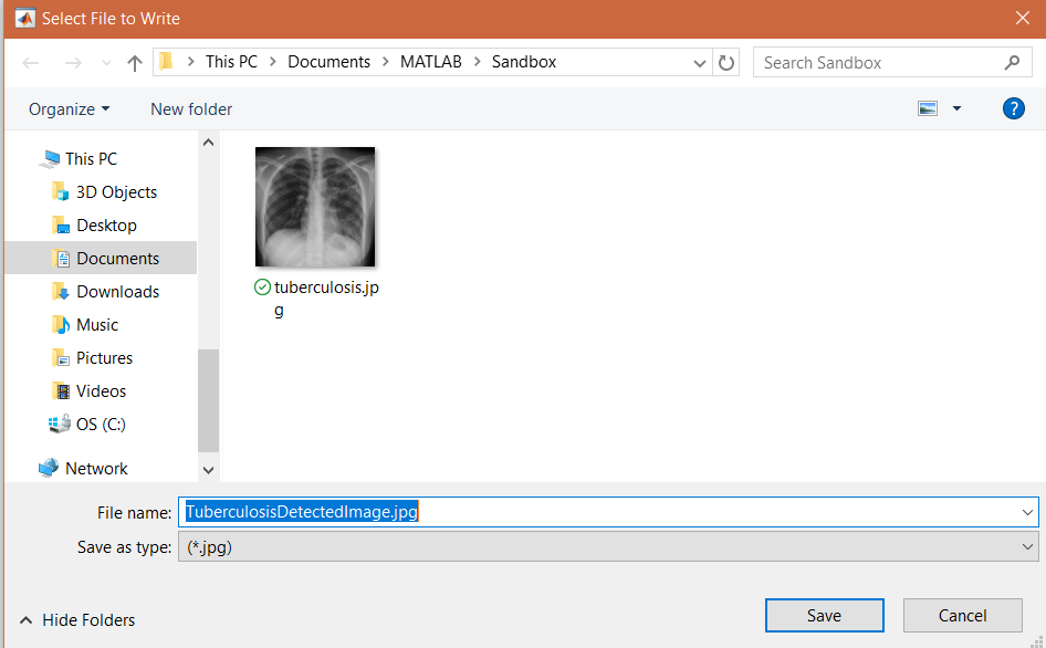
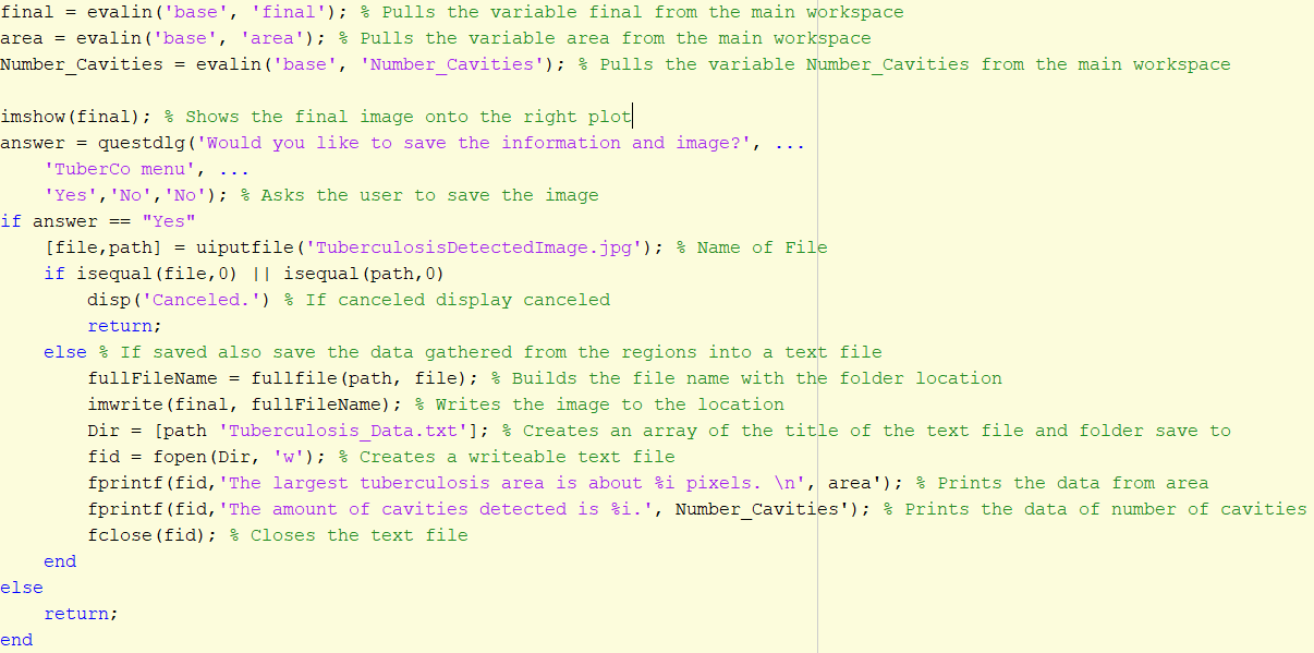
The main code is primarily done, but we wanted to provide the user the option to save the data that was created with this code. We want to be able to save the image with the locations of the cavities along with the data about the number of cavities and the area of the largest cavity.
First, we have to restore all variables that we saved into our base workspace from the last code, which does not mean much now but will be extremely helpful when we combine it with the GUI!
final = evalin('base', 'final'); % Pulls the variable final from the main workspace
area = evalin('base', 'area'); % Pulls the variable area from the main workspace
Number_Cavities = evalin('base', 'Number_Cavities'); % Pulls the variable Number_Cavities from the main workspace
-----------------------------------------------------------------------------------------------
The evalin function restores the data from the indicated workspace, base, into the current workspace. We can show our final figure as an image this time using:
imshow(final); % Shows the final image onto the right plot
-----------------------------------------------------------------------------------------------
We want the user to have the choice on whether they want to save the information or now, so we opted to use another message box. Instead of having the user input a value this time, we will have the user either select “yes” or “no”. This can be completed using the function questdlg:
answer = questdlg('Would you like to save the information and image?', ... 'TuberCo menu', ... 'Yes','No','No'); % Asks the user to save the image
if answer == "Yes"
[file,path] = uiputfile('TuberculosisDetectedImage.jpg'); % Name of File
if isequal(file,0) || isequal(path,0)
disp('Canceled.') % If canceled display canceled
return;
-----------------------------------------------------------------------------------------------
The function allows you to input a title, a message, and choices. The last choice has to be written twice for it to properly work and appear as a single button. This value is saved as a string to the variable answer. We do need to recognize this variable so we have to use a character array instead of a string to recognize the entire phrase “Yes”. We then give the user the option to pick the save location using uiputfile and of course allow the dialog to be canceled as well. We now want to save the image and also save the data into a text file. We put all of this information into the else statement when it is not canceled as below:
else % If saved also save the data gathered from the regions into a text file
fullFileName = fullfile(path, file); % Builds the file name with the folder location
imwrite(final, fullFileName); % Writes the image to the location
Dir = [path 'Tuberculosis_Data.txt']; % Creates an array of the title of the text file and folder save to
fid = fopen(Dir, 'w'); % Creates a writeable text file
fprintf(fid,'The largest tuberculosis area is about %i pixels. \n', area'); % Prints the data from area
fprintf(fid,'The amount of cavities detected is %i.', Number_Cavities'); % Prints the data of number of cavities
fclose(fid); % Closes the text file
end
else
return;
end
-----------------------------------------------------------------------------------------------
The final image is saved using imwrite with the file name and path from uiputfile. To create a text file with the data, we create an array with variable Dir that contains the path location and a file name. We open a writeable text file using fopen with it set to write mode, the ‘w’. We use this to print whatever we want into the file using fprintf, and include the variables with the data. As well, we include a return option if the user never wanted to save in the first place.
Creating the GUI
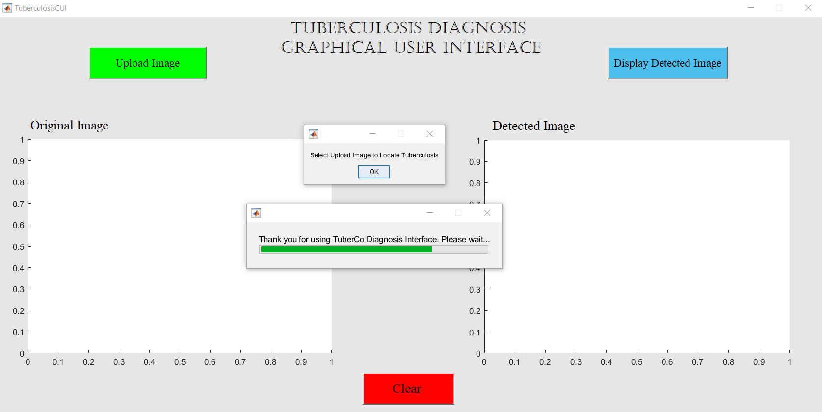
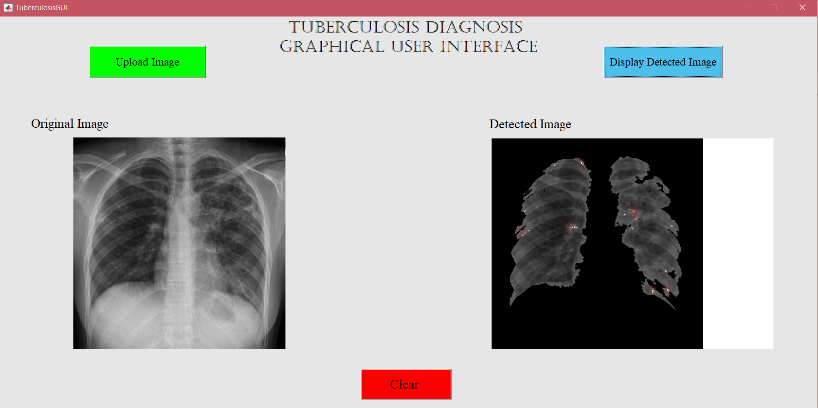
Using the built in GUIDE program in MATLAB is great way to build your first GUI. This program can be opened by typing guide in the command window. Any of the buttons that are placed will have a code made automatically that can be used with any of our previous code. Below is the exact code that we have for our GUI setup, but you will also need the .fig file that is attached at the bottom of the page.
Any of the colors, fonts, and sizes can also be edited with the GUIDE function. This change will edit the .fig file, which contains the information about the GUI itself. The .m file contains the information about what each of the different button does and how it runs.
Section 1: Initializes Waitbar
This section creates a waitbar that says "Thank you for using TuberCo Diagnosis Interface. Please wait...". The function closes after 1000 steps of the for loop.
h = waitbar(0,'Thank you for using TuberCo Diagnosis Interface. Please wait...'); % Create a wait bar to notify user to wait
steps = 1000; % Uses waitbar to wait about a second for GUI to load
for step = 1:steps % Run for loop till it increments to 1000
waitbar(step / steps) % Increases the loading bar at a rate of 1/1000
end
close(h) % Closes waitbar
------------------------------------------------------------------------------------------------------------------
Section 2: Create a Message Box to Tell the User
We want to tell the user how to start the code and to do so we use the following commands. Most of it is automatically written, except the msgbox command which is what we coded into the start of the program.
function varargout = TuberculosisGUI_OutputFcn(hObject, eventdata, handles) %Varargout is varying arguments which is basically a GUI variable.
% Get default command line output from handles structure
varargout{1} = handles.output; %varargout creates an implicit variable that outputs two different axes on the GUI. % Also, hObject is a GUIDE variable that is used when inserting static text, pushbuttons, or images.
g = msgbox('Select Upload Image to Locate Tuberculosis'); % Tells user to press the Upload button to start program
------------------------------------------------------------------------------------------------------------------
Section 3: Create a Push Button to Start the Code
This part of the GUI code initializes a pushbutton to upload a file using uigetfile and selects the type of file and to upload the file and run the code. This code also includes the previous code we made that includes reading the image file and displaying the image.
function pushbutton1_Callback(hObject, eventdata, handles) % This function is created when placing the first pushbutton which is "Upload Image"
Dir = [folder file]; % Creates an array of the folder location and the file name
grayImage = imread(Dir); % Reads the selected file from the folder with Dir
axes(handles.axes1);% Displays on the first plot which is the left plot
imshow(Dir) % Shows the image selected on the left plot
--------------------------------------------------------------------------------------------------------------------
Section 4: Display the Detected Image
This section of the GUI code calls on a pushbutton callback function that displays an object. After the image is shown, a question dialog box appears and asks would you like to save the image and if yes is selected, user can save the image. This section of the code would feature the evalin functions to recall the variables as well as indicating which axis to plot the image on.
function pushbutton2_Callback(hObject, eventdata, handles) % This function is created when placing the second pushbutton which is "Display Detected Image"
axes(handles.axes2); % Selects the second plot a.k.a the right plot
imshow(final); % Shows the final image onto the right plot
---------------------------------------------------------------------------------------------------------------------
Section 5: Clear Axes
This section of the GUI code initializes the third pushbutton which clears the axes and initializes the GUI for other users to upload their photos and test and diagnose tuberculosis. We simply coded to tell the certain axis to clear using cla reset.
function pushbutton3_Callback(hObject, eventdata, handles) % This function is created when placing the third pushbutton which is "Clear"
axes(handles.axes1) % Selectes the left axis
hold off; % Wait to clear
cla reset; % Clears the plot
axes(handles.axes2); % Selects the right axis
hold off; % Wait to clear
cla reset; % Clears the plot
-------------------------------------------------------------------------------------------------------------------
Combining the Tuberculosis Code With the GUI Code
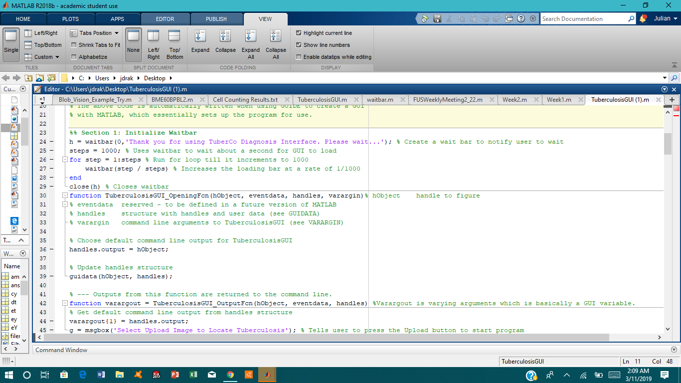
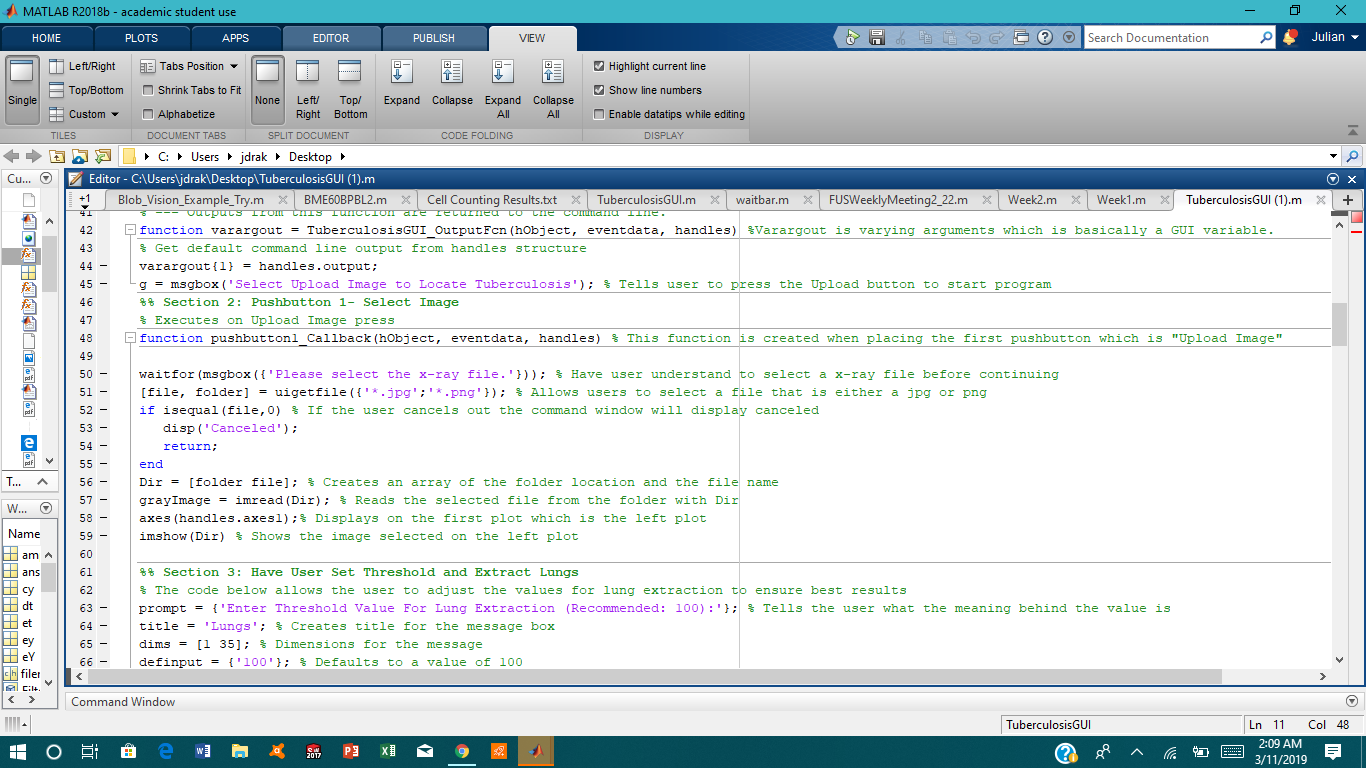
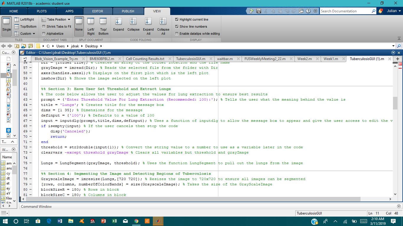
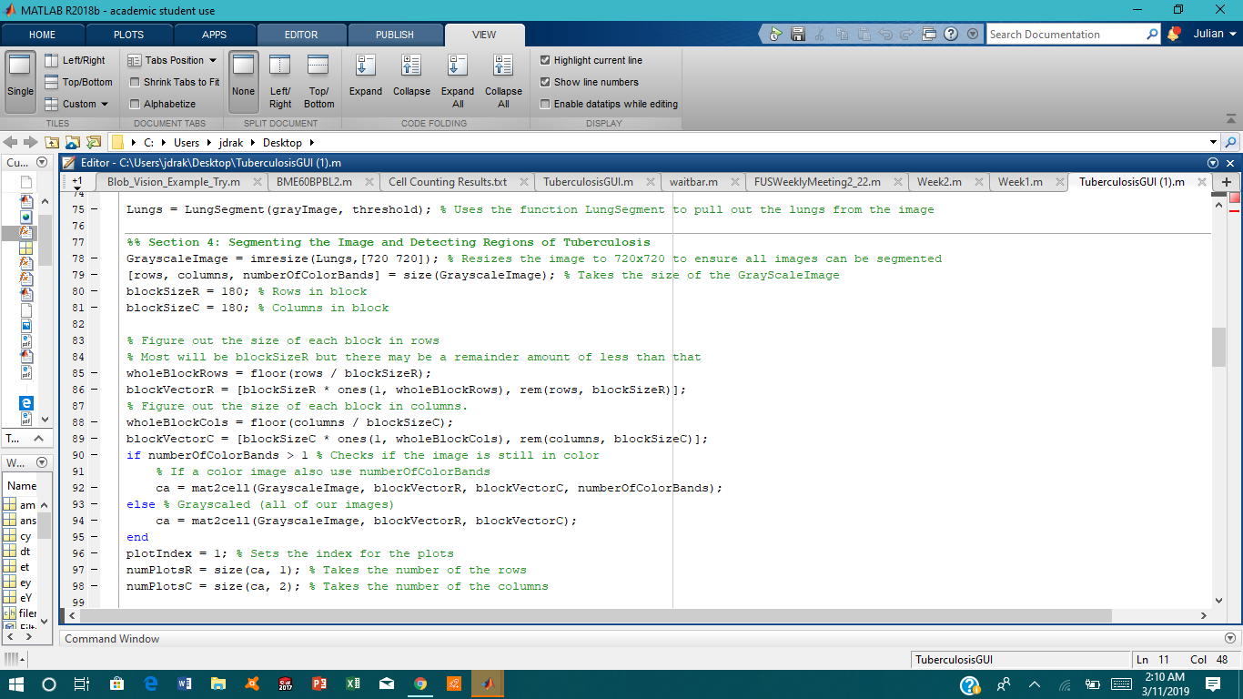
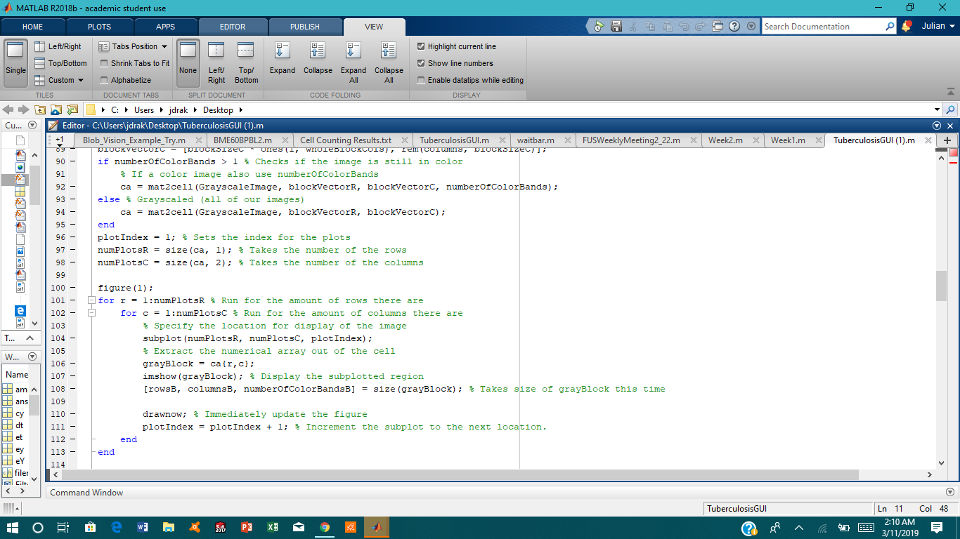
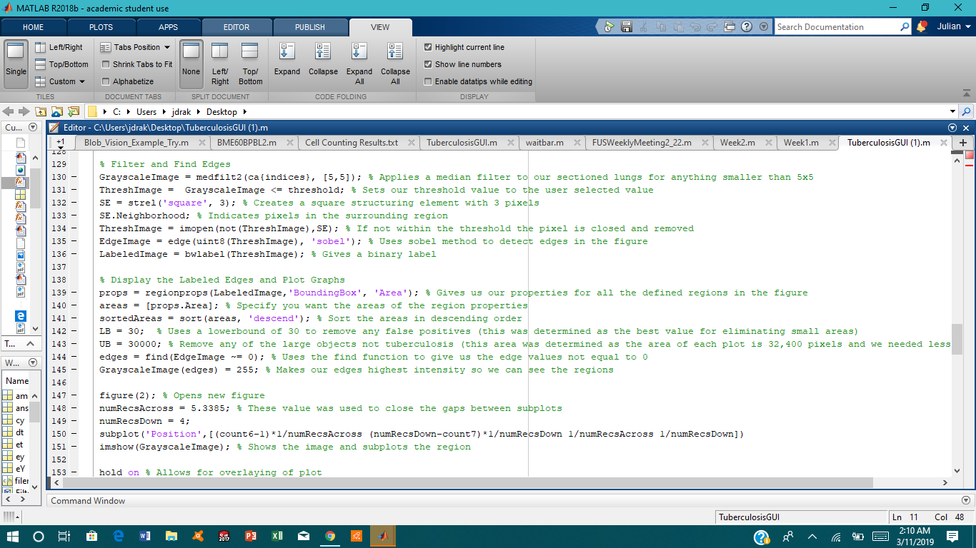
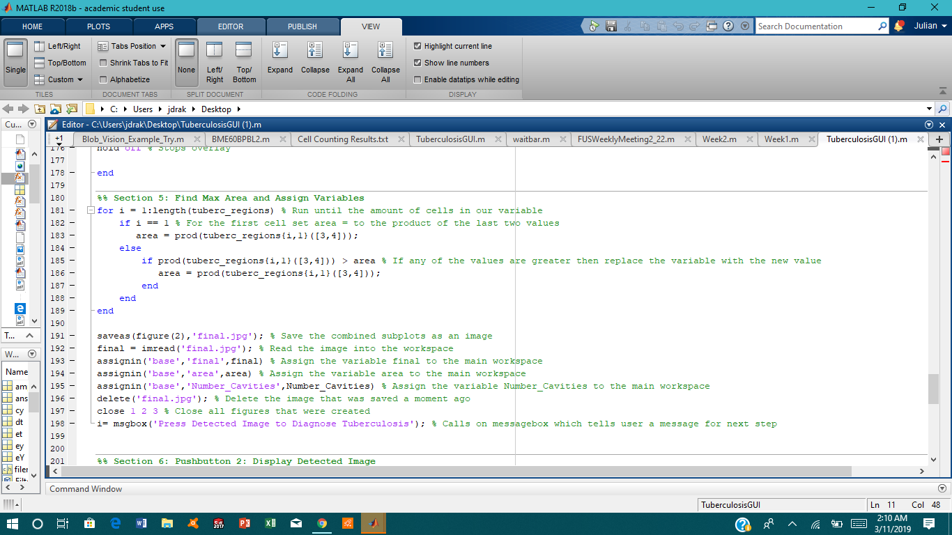
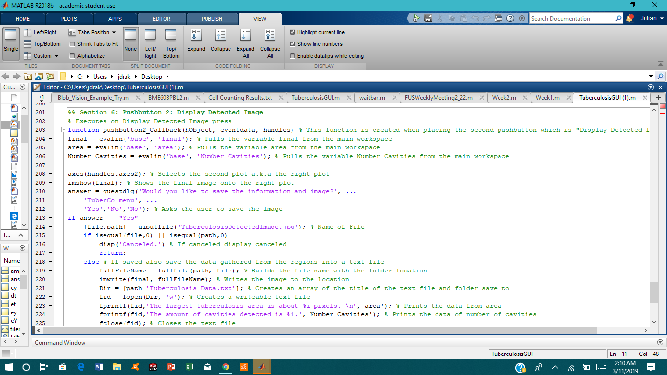
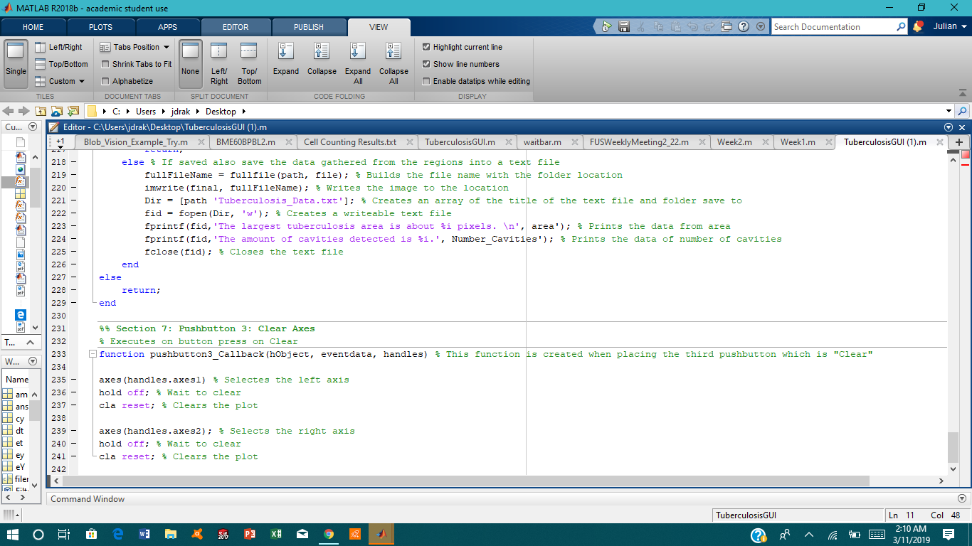
The code that is displayed is a compilation of the GUI code and the tuberculosis diagnostic code. Each section is slightly modified but it is a compilation of all the sections of this instructables. When combining the code make sure to put the code you want to run into each of the functions that correspond to a specific button. As well, the variables will not transfer from function to function, but it is a good thing we already coded a way to import and export the variables from the main workspace when needed!
The pictures of this section showcase how exactly we combine the GUI code with the main code to make it run how we desired it to do.
Congratulations! and Final Thoughts

Thank you for walking with us through this journey and hopefully you learned at least something. Ourselves learned a lot from this process and are proud on what we could accomplish in the time frame we had. Of course, if we had more time there could have been other techniques or methods we would have implemented. This code is definitely a starting point for any future projects and feel free to adapt this code for your future needs. Always remember to have fun!
Any items or code that was used is located below this section with one of the pictures used is located above. Feel free to download or start the code from the scratch!
References
Betsy, Antony, and P K Nizar Banu. “Lung Tuberculosis Detection Using X-Ray Images.” International Journal of Applied Engineering Research, vol. 12, no. Number 24 (2017), 2017, pp. 15196–15201.
“Gobjects.” Reconstructing an Image from Projection Data - MATLAB & Simulink Example, Mathworks, www.mathworks.com/help/matlab/ref/gobjects.html.
Horváth, Péter. “MatLab for Biologists.” Light Microscopy Centre ETH Zurich, 5 May 2008, group.szbk.u-szeged.hu/sysbiol/data/peter-horvath-lab/education/matlab/matlab_lect_3.pdf.
“imresize.” Reconstructing an Image from Projection Data - MATLAB & Simulink Example, Mathworks, www.mathworks.com/help/images/ref/imresize.html.
MathWorks. “Reconstructing an Image from Projection Data - MATLAB & Simulink Example.” Reconstructing an Image from Projection Data - MATLAB & Simulink Example, www.mathworks.com/help/images/ref/imresize.html.
“Mohammad Ayoub .” Reconstructing an Image from Projection Data - MATLAB & Simulink Example, www.mathworks.com/help/images/ref/imresize.html. Gui-how-can-i-prevent-a-push-button-from-re-initializing-my-variables.
“How Can Imfill an Image with a Lot of Edge?” MathWorks, 8 Sept. 2014, www.mathworks.com/help/images/ref/imresize.html.
Patil, S A. “TEXTURE ANALYSIS OF TB X-RAY IMAGES USING IMAGE PROCESSING TECHNIQUES.” Journal of Biomedical and Bioengineering, vol. 3, no. 1, ser. 2012, 9 Mar. 2012, pp. 53–56. 2012, doi:10.9735/0976-8084.
Reconstructing an Image from Projection Data - MATLAB & Simulink Example, www.mathworks.com/help/images/ref/imresize.html.
Shinobii. “MATLAB Save Image from GUI Using Push Button.” Stack Overflow, stackoverflow.com/questions/11671892/matlab-save-image-from-gui-using-push-button
“Split Image into Blocks.” MATLAB Wiki, matlab.fandom.com/wiki/Split_image_into_blocks.
“Tuberculosis Chest X-Ray Image Data Sets – Communications Engineering Branch.” U.S. National Library of Medicine, National Institutes of Health, ceb.nlm.nih.gov/repositories/tuberculosis-chest-x-ray-image-data-sets/.