Simple Organization of Raw Data: Harnessing Pivot Tables in Excel for Efficiency
by akaiser1125 in Workshop > Organizing
222 Views, 3 Favorites, 0 Comments
Simple Organization of Raw Data: Harnessing Pivot Tables in Excel for Efficiency

Efficiency is paramount when managing and analyzing complex sets of raw data. The larger the data set, the harder organization of said data becomes. That is, until you master a feature in Microsoft Excel called Pivot Tables. Pivot tables are dynamic and allow you to quickly rearrange and organize raw data. Once you have a pivot table made, you can then quickly gather insights, summaries, and much more about the data. Pivot tables are important because they provide a systematic method of managing and analyzing raw data. Mastery of pivot tables opens the door to the necessary data-driven insights needed to make informed decisions in your business.
Supplies
You will need:
A charged laptop (pricing as low as $102.99 from Best Buy)
A wireless mouse (pricing as low as $9.99 from Best Buy)
Microsoft 365 Personal (purchase digitally for $69.99 from the Microsoft Store)
Disclaimer: This presentation is for educational and informational purposes only. Though I will show you how to create a pivot table, revealing an easy and efficient way to organize raw data, it is necessary to note that the effectiveness of this tool depends entirely on the validity of the data set in use. Users are responsible for evaluating the validity of any data sets they may use. When using pivot tables in Microsoft Excel, users must acknowledge and accept the inherent risks of using data that they did not collect themselves. The creator of this presentation disclaims any liability for damages or loses arising from the use of pivot tables.
This presentation is made with the assumption that viewers know how to operate a laptop and that the user will have Microsoft 365 Personal already installed on their device prior to Step 1 of this presentation. A wireless mouse is not a necessity for using Pivot Tables in excel. Pivot tables in Microsoft Excel can be created by using the built-in mouse-pad of a laptop. I personally recommend the use of a wireless mouse because it is much easier and far more efficient to work in Excel with one, rather than using the built in mouse-pad of the laptop
Locate the Microsoft Excel Application on the Laptop and Open It

Once you are signed into your laptop and at the main home screen, find the icon for Excel. You may need to search for it, as shown in the photo above. Once you locate it, double click on it to open the App.
Open the Spreadsheet Containing the Data You Will Use

Once Excel is open, use the task bar at the top of Excel to click file, open, and choose the spreadsheet containing the data set that you would like to turn into a pivot table.
Highlight ALL of the Data in the Spreadsheet, Including Column/row Titles
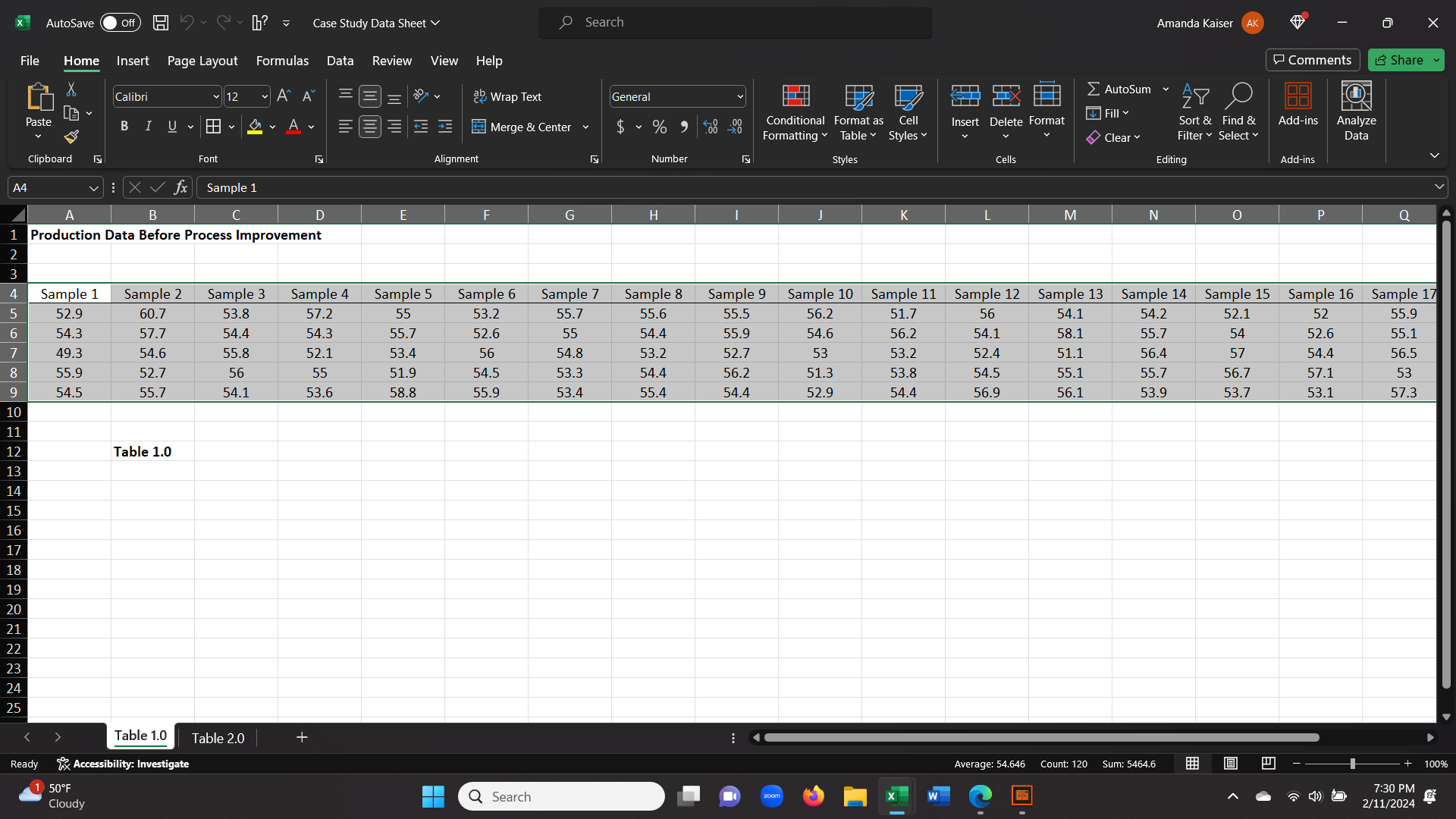
Highlight all of the data in the spreadsheet by click on the first cell and dragging your cursor to the bottom most cell on the right side of the spreadsheet. Do not let go of the mouse once you click it until you have all the data highlighted. Be sure to include any row or column titles in the highlight.
Go to the "insert" Tab
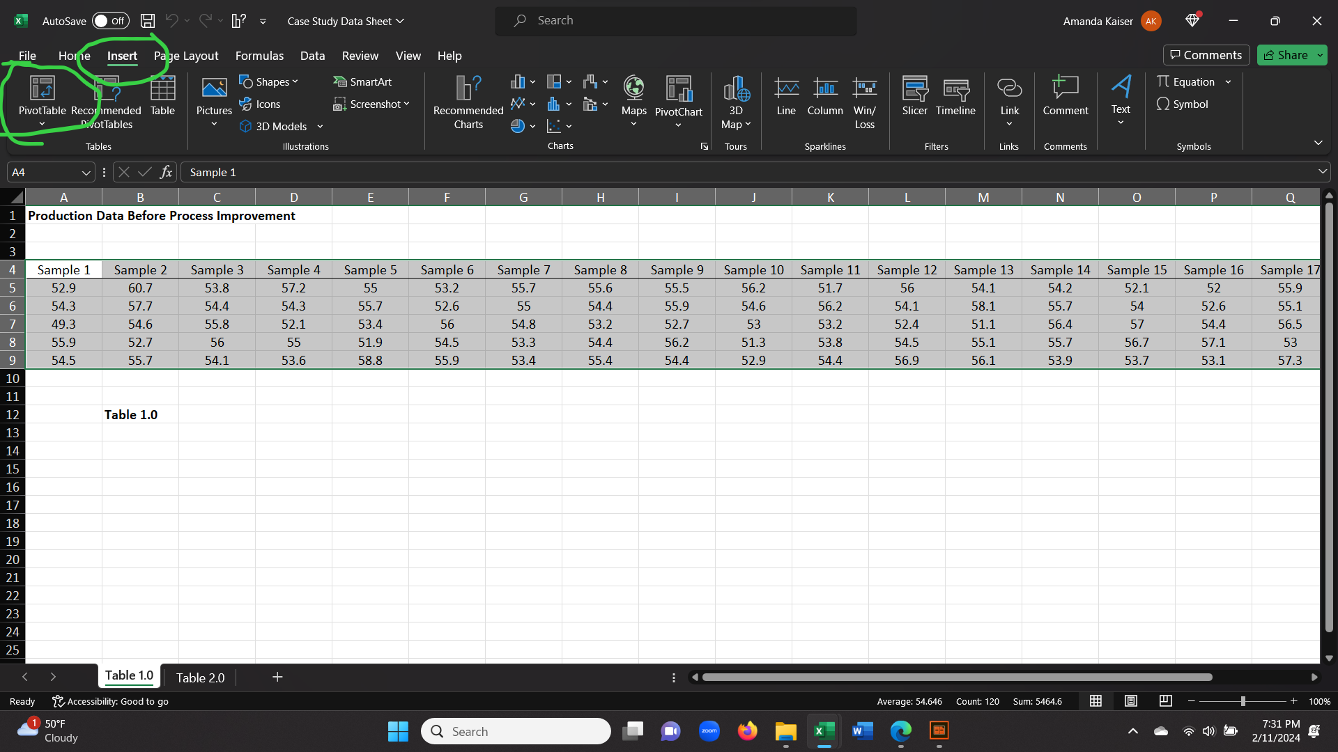
Click on the "Insert" tab that is located towards the top of the App on the left-hand side.
Choose "Pivot Table" and Click "ok" on the Message Box That Pops Up
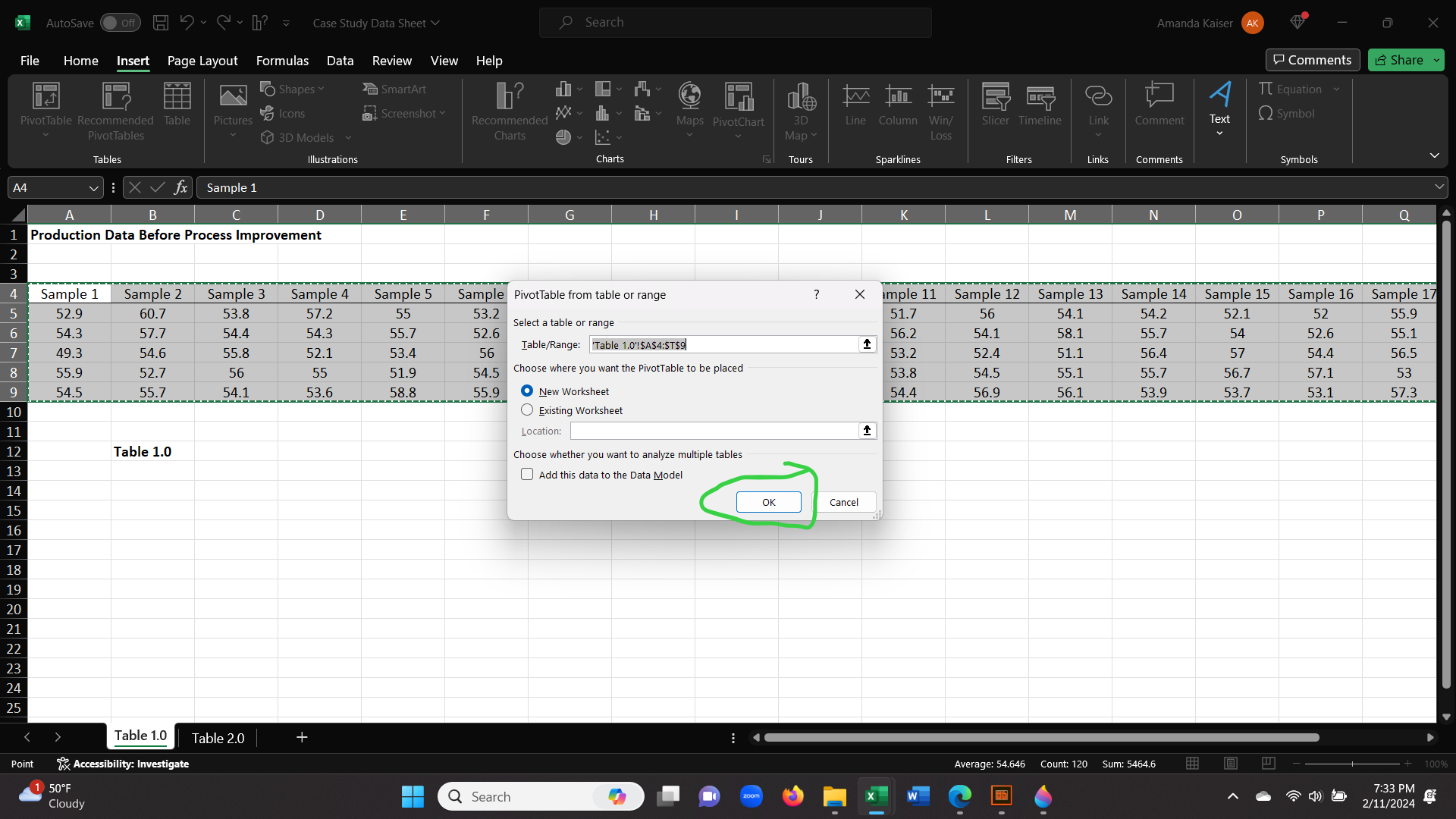
Click on "Pivot Table". A message box will pop on your screen asking you turn confirm the data range that will go into your pivot table. All you have to do is click "ok".
Drag and Drop Data Into the "Fields" Boxes
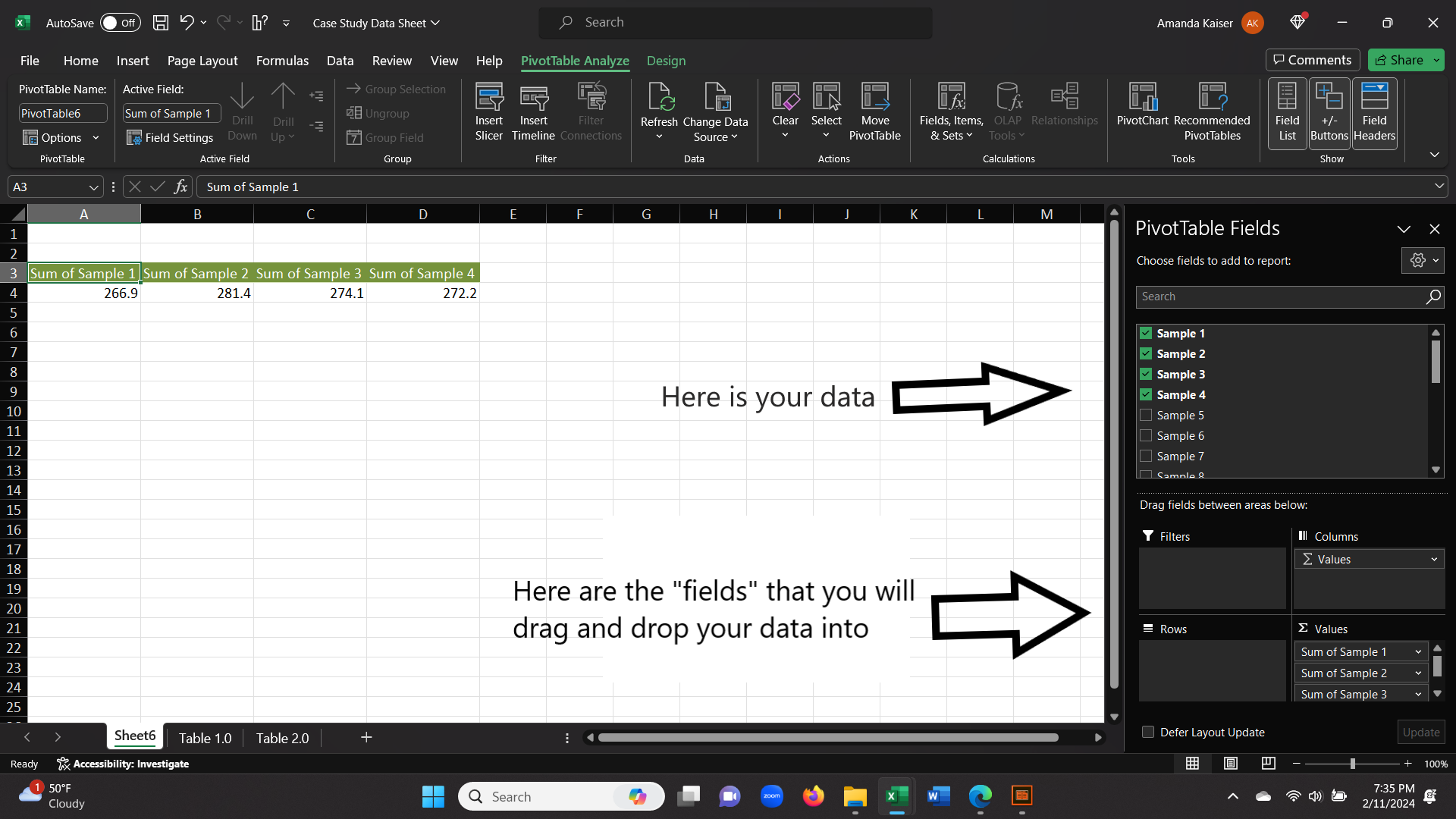
Next you will drag and drop your data that is located on the left side on your screen into the "fields" below. You can choose to include or disclude any data. Due to the nature of my data set dragging and dropping data into the "values" field will result in Excel automatically figuring the sum of all data points per sample.
Keep in mind that different data sets will return different options and looks of a pivot table. If you are unsure of where to drag and drop data for the best use, instead of clicking "Pivot Table" in Step 5, you can choose the icon to the right of it titled "Recommended Pivot Tables". Clicking that will return a pop-up window that lets you explore the possible pivot tables for the data set.
Analyze Your Data Now That It Is Organized
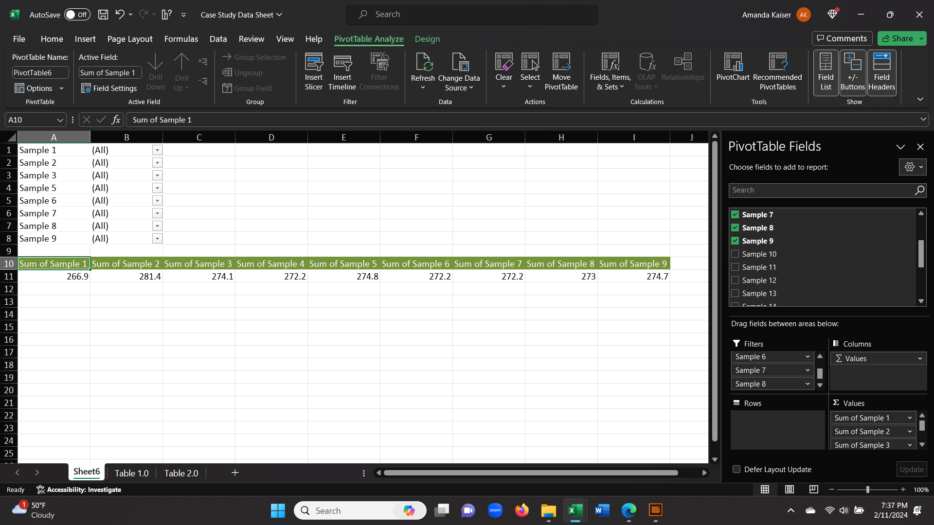
You can drag and drop your data into the "filter" field and Excel will create a dropdown for each sample, allowing you to go back and see all data points.
Now that your pivot table is set up, you can easily analyze your data without having to splice-n-dice or enter a single formula! The pivot table that I have created here allows me to see the sum of each sample. I included the drop-down options for each sample as well. This allows me to look back at each data point that makes up the sum for Sample 1, Sample 2, etc. Without the pivot table, I would have had to enter the SUM formula individually for each Sample. The drop-down menus make it so I do not need to switch back and forth between spreadsheets. The final product allows quick analysis of the sum of each Sample and without having to go back to the raw data spreadsheet, I can use the drop-down box to view all data points included in each sample.
Example

I have included this video as a means of seeing all of the steps together. I also see value in watching this video because the data set is different from the one I used, giving the viewer a deeper understanding of all that can be done using a pivot table. Different data sets look different in a pivot table!