PID and Feedforward Controller for Precise Trajectory Following
by yankaih in Circuits > Robots
910 Views, 5 Favorites, 0 Comments
PID and Feedforward Controller for Precise Trajectory Following

The goal of this project is to get a two-wheeled robot (with a caster) to travel to a coordinate in the world frame as precisely and quickly as possible. We achieved this by generating a reference trajectory based off of a cubic spiral, using encoder readings to calculate the robot's current position in the world frame, and using feedforward and PID to adjust the robot's position so that it approaches the reference trajectory.
Steps 3 to 8 below document our methods for tuning this system and our results in video form with explanations.
Supplies
- Matlab (with ROS and Statistics and Machine Learning Toolkits)
- Matlab Raspbot Simulation API File (From 16-362 Website)
- Raspbot
Setting Up the Robot Simulation Environment
- Install Matlab (check the ROS and Statistics and Machine Learning Toolkits)
- Download the Matlab Raspbot Simulation API File from the 16-362 course website
Understanding Robot Capabilities and Dynamics
These assumptions are made by the Matlab Raspbot Simulation API:
The nominal wheelbase is 9cm. Diameter of the robot is ~12cm
Maximum speed - 0.3 m/s. This is the maximum speed the robot API will accept for either wheel. Beyond that, the API should throw an error message and not cause the robot to respond.
Max acceleration - 10 m/s/s. This is enforced by the PID driver on the robot, not the API. Any higher accelerations cause unstable PID control.
Encoder message rate - 50Hz. These messages are sent by the robot automatically. The simulator may be slower (say 30 Hz) because it is also using up your CPU cycles to do the simulation.
Velocity commands maximum rate - 50 Hz. The API will send these to the robot no faster than 50 Hz.
Citations: https://www.andrew.cmu.edu/course/16-362-862/Docs/robots.html
Tune P-Controller to Travel 10 Cm in a Straight Line (Kp=3)
.png)

Using a proportional controller, we calculated the error as follows:
error_distance = goalposition - current position
where the current position is determined by integrating the encoder readings. That error (distance to the goal) is then multiplied with the proportional gain to produce a velocity command (capped by 0.3 m/s) that we send to the robot.
To calculate the velocity command we do:
command = Kp*error
We started with a Kp of 3, and the robot speeds up initially (error is big) and slows down towards the end (error is small), and does not overshoot 10 centimeters. However, it approaches the target relatively slow (took about 1 second).
Tune P-Controller to Travel 10 Cm in a Straight Line (Kp=13)

We wanted to see if we can get the robot to reach the target position faster using the proportional gain. We expected there to be oscillations and overshoot as a result, and that is exactly what we found when we used a Kp of 13:
The controller made the robot move 10 centimeters within 0.5 seconds, but the large overshoot and enduring oscillations made the result unusable.
Tune PD-Controller to Travel 10 Cm in a Straight Line (Kp=13, Kd=0.6)
After experimenting with a few derivative gains, we found the optimal Kd to be 0.6. If we set the derivative gain lower and underdamp the system, then the robot oscillates around the destination for too long. If we set the derivative gain much higher and overdamp the system, then the robot approaches the goal slowly.
To calculate the velocity command we now do:
command = Kp*error + Kd*(change in error)
where change in error is calculated by differentiating the encoder readings between each time step.
As you can see in the video, there is a small overshoot but the robot gets there decently fast at around 0.5 seconds.
Try a Feedforward Controller to Travel 10 Cm in a Straight Line

Since we know that the fastest we can make the robot accelerate is 10 m/s/s and the robot's max velocity is 0.3 m/s, we can create a trapezoidal velocity profile. Robot velocity command starts at zero and increases at a rate of 10 m/s/s, then plateaus at 0.3 m/s, before decelerating at a rate of 10m/s/s back to zero. Given the distance we need to travel, we can calculate how long the robot needs to accelerate, maintain max speed, and decelerate for (integration of the trapezoid should equal the distance).
In addition to trying a feedforward controller, we added a 0.083 second delay between when velocity commands are sent and when the robot starts moving.
As you can see in the video, the robot reaches the target destination relatively fast at 0.05 seconds, but does not correct its position at the end because there is no feedback.
Combining Feedforward and PID
Benefit of Feedforward: Does not produce unreasonable command velocities and gets to the goal relatively fast
Disadvantage of Feedforward: Does not adjust itself so we get to where we want exactly
Benefit of PID: Adjusts the command based on the existing error between where we are and where we want to be
Disadvantage of PID: May produce unreasonable command velocities (ex: if the distance is large, resulting in oscillations/overshoot)
The benefits of one system cancel the disadvantage of the other system, so we decided to combine feedforward with PID to get the robot to travel to where we want precisely. This time, however, our error is not the distance from current position to goal position. Instead it is:
error = reference position (where we should be according to feedforward) - actual position from encoders
pid_command = Kp*error + Kd*(change in error)
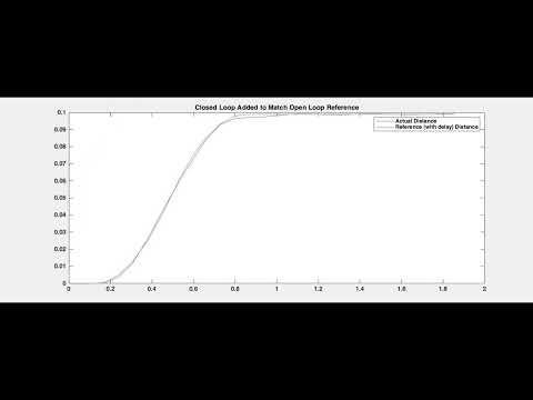
As you can see in the video, the robot gets to the goal position quickly (0.5 seconds) by sending in the feedforward velocity command + the pid_command. In the plot at the end of this video, you can see small oscillations of actual around the reference, but it generally follows the reference closely. This is the PID part of the controller catching up with the feedforward reference position.
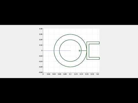
Not Just a Straight Line!

A robot that can only move forward is not very useful. Therefore, we implemented a cubic spiral trajectory generator for the robot to use. Given the cubic spiral trajectory, we used a pure pursuit algorithm where, at each timestep, the robot looks forward in the trajectory, and generates a velocity to get to the lookahead point.
By using the feedfoward + feedback controller in step 7, we calculate the velocity V. Then we can calculate the left and right wheel velocities as follows:
L_velocity = V*(2 + C*T)/2
R_velocity = V*(2 - C*T)/2
where C = curvature, T = track width
As you can see in the video where we gave three coordinates in the world frame for the robot to travel to, the robot successfully follows the reference trajectory very closely using this algorithm.
Citation/Reference We Used To Construct the Cubic Spiral Trajectory:
- Liang, Tzu-Chen and Jing-Sin Liu. “A Path Planning Method Using Cubic Spiral with Curvature Constraint.” (2002).
- 16-362 Lecture #7 Slides
Discussion
From our project, we learned of these two main ideas:
- Control method can be generalized to following a more complex trajectory
- Combination of feedback and feedforward results in very close trajectory following
1) We realized that using a controller to generate velocity commands for a robot to move in a straight line towards its goal can be quickly generalized to trajectories that turn smoothly (such as in a cubic spiral trajectory).
2) We learned to appreciate the combination of open loop and closed loop aspects in a controller since the open loop generates very close to ideal commands (in simpler systems like this one) and the closed loop closes any gaps between the reality and the simulation.
Limitations of our project include the fact that we were treating the robot position derived from the encoder readings as the robot's actual position. In reality, the encoder could have noise and errors that accumulate over time. This problem can be addressed by using sensors such as lidar (also included on the raspbot) and localization techniques to verify and reset the position of the robot periodically. By doing these adjustments, the robot can calculate a more accurate error, thus resulting in better velocity commands when applying controller gains.