Monthly Budget Planner

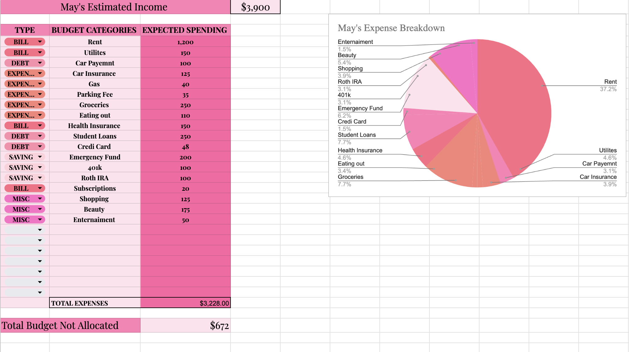
Here is a completed Digital Budget Tracker

Open Google Sheets by going to https://sheets.google.com

Click on "Blank" to create new spreadsheet

In the first row of the spreadsheet, create headers for your data:

• In cell A1 enter May's Estimated Income
• In cell D1 enter your month's income
• Move down to row 3
• In cell A3 enter "TYPE"
• In cell B3 enter "BUDGET CATEGORIES"
• In cell C3 enter "EXPECTED SPENDING"
• In cell B29 enter "TOTAL EXPENSES
• In cell A31 enter "Total Budget Not Allocated

Select the first row.

Click on the Bold button (or press `Ctrl + B`).

Change the background color of the headers for better visibility by clicking the Fill color button and selecting a color.

Adjust the column widths to fit the content by double-clicking the right edge of each column header.

For your budget table(where your data will be) underneath the TYPE and BUDGET CATEGORIES headers select cells A4: B29 and change the background color

Then under the Expected Spending header select cells C4:C29 and change the background color

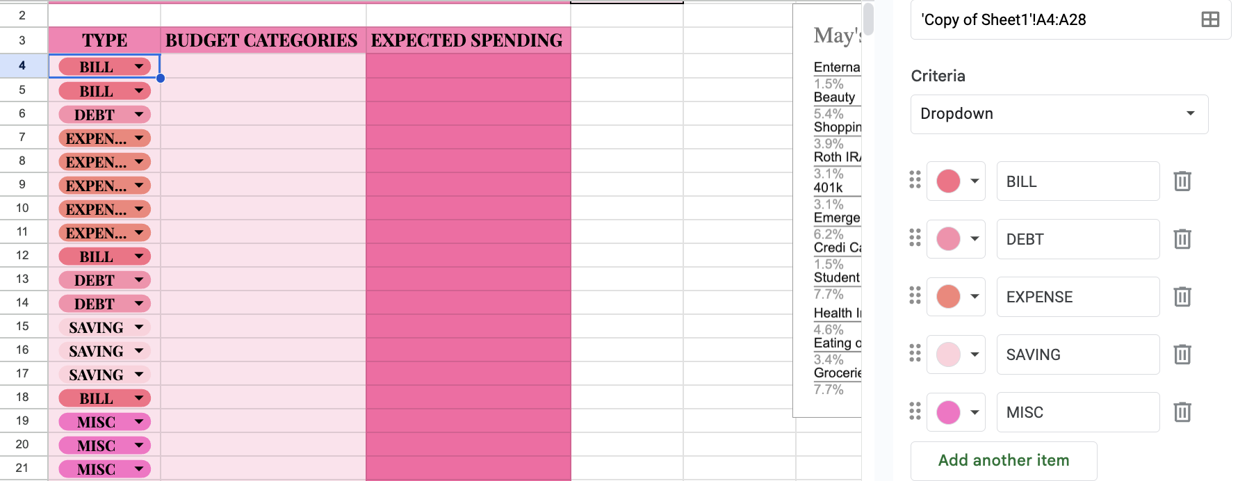
To ensure consistency in your categories, you can use data validation.

Select the cells under the "TYPE" column (e.g., A4:A28).

Go to `Data` > `Data validation`.

In the "Criteria" field, select `List of items` and enter your categories (e.g., Bill, Debt, Expense, Saving ).

(Optional) To add color to your data-validated categories simply click the blank circle and press customize to add colors to each of your labels

Click `Save`

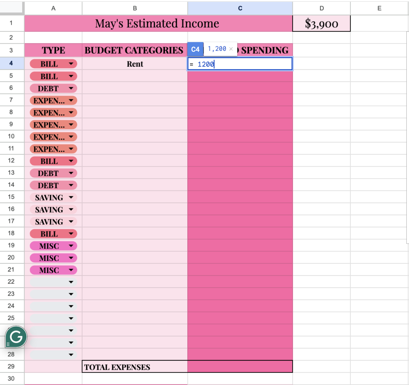
Input your monthly transactions under each header to get started. For example:

• Cell A4: Bill
• Cell B4: Rent
• Cell C4: =1,200
• Cell A5: Bill
• Cell B5: Utilities
• Cell C5: =150
• Cell A6: Debt
• Cell B6: Car Payment
• Cell C6 =100
• Continue inputting your monthly transactions untill complete

*when inputting values under the "Expected Spending" column don't forget to add = then amount to ensure accurate total expenses

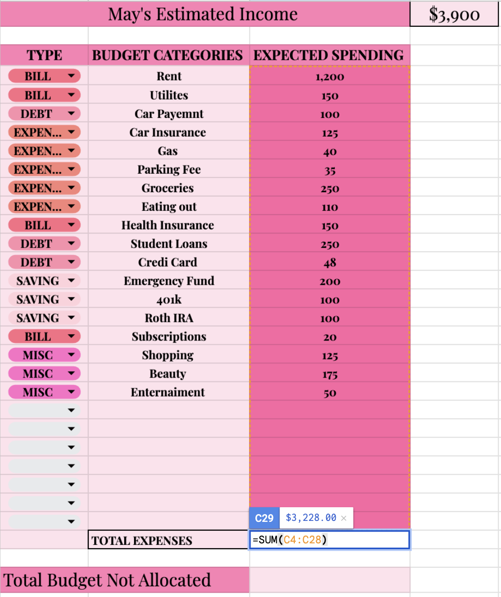
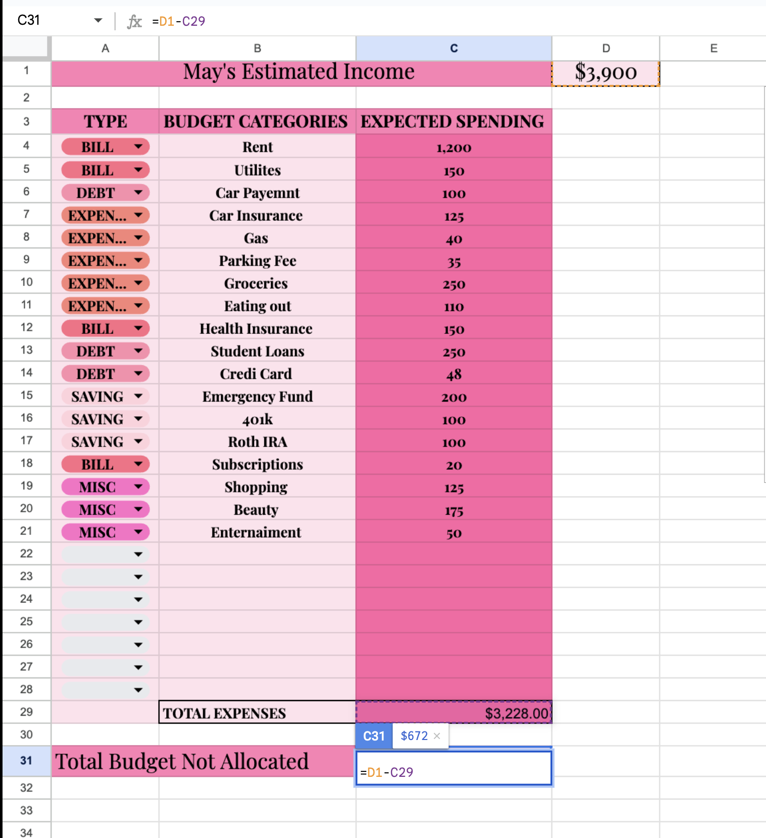
In cell C29 (adjacent to the "TOTAL EXPENSES" cell) input formula =sum(C4:C28)

• This formula adds individual cell ranges and calculates the sum

Move down to row 31 and in cell C31 =D1-C29

• This formula is your total expense from your total income

Select the data range you want to visualize (e.g., your income and expenses data).

Go to `Insert` > `Chart`.

Choose the chart type that best represents your data (e.g., pie chart for category breakdown, line chart for trends over time).

Customize the chart as needed.

 Click on `File` > `Save` to ensure your data is saved.

To share your budget planner with others, click on `Share` in the top-right corner, enter the email addresses, and set the appropriate permissions (e.g., view or edit).