Low Cost PIV System
by BrownUniversityENGN in Workshop > Science
6074 Views, 5 Favorites, 0 Comments
Low Cost PIV System
The cheapest, most accessible, and easily reproducible PIV system!
Compared to the literature we reviewed, we were able to develop a system that is significantly cheaper. We believe the cost that's in the low hundreds is unparalleled and we are confident we bought some of the cheapest options while maintaining great functionality. With the help of open-source software, we also believe that for the incredibly cheap system, our system was easy to manufacture and work around with, making this project a great success.
Supplies
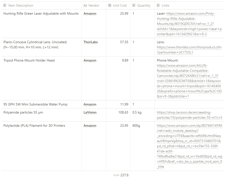
- 1 Plano-Concave Cylindrical Lens. Uncoated. f = -15.00 mm, H = 10 mm, L = 12 mm
- 1 Pinty Hunting Rifle Green Laser Sight Dot Scope Adjustable with Mounts
- 1 Tripod Phone Mount
- 1 5W Mini Submersible Water Pump
- 1 4x8x16 Acrylic Tank 6.85 cubic inches polylactide (PLA)
- 2 screws (lens mount)
- 2 ¼ - 20 threaded rod (laser mount)
- 1 tablespoon 50-micron, silver-coated hollow ceramic spheres
- 1 8x16 White Construction Paper
- 1 Phone Camera (capabilities to capture 120 fps in slow motion)
- Open Source PIVLab software
The total cost for purchasing these materials is $237.80. There is an abundance of polyamide particles and PLA Filament for 3D Printers, thus the experimental setup can be produced multiple times for many trials.
Materials and CAD Models
MATLAB Scripts
1. Get the video to get black and white frames in one folder using prepre.m
Some video we took is also available for download (we use this filename in prepre.m if you want to test out how that one works), but you can always edit the filepath in prepre.m to work with any video you take.
2. Calculate the scale of your video from pixels to meters using calculate_scale.m
You must have a reference object with a known distance in your video. We use the pump nozzle as our reference object, selected two points across the diameter of the nozzle, and used the known diameter to calculate the scale for our images. You may also include a ruler in your video (which would work just as well).
3. Read text files of the vector data created by PIVlab using txtprocessing.m
You can save text files from PIVlab by going to File—>Export—>txt
Note: Instructables does not allow MATLAB (.m) files to be uploaded. The code is instead presented in plain text form.
3D Print
3D Print the Laser/Lens Mount and Tank Mount by downloading the files and adjusting necessary printer settings.
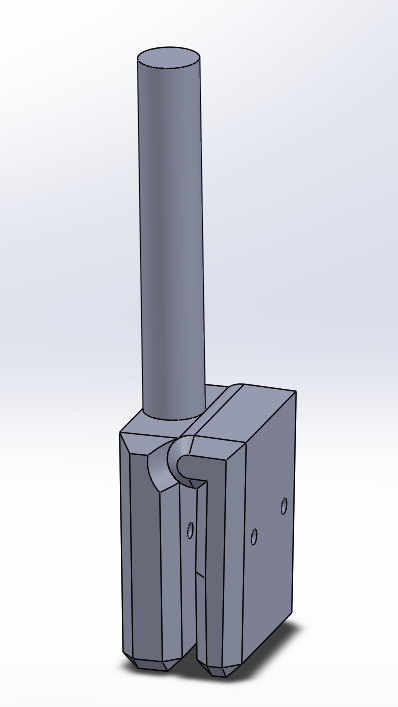
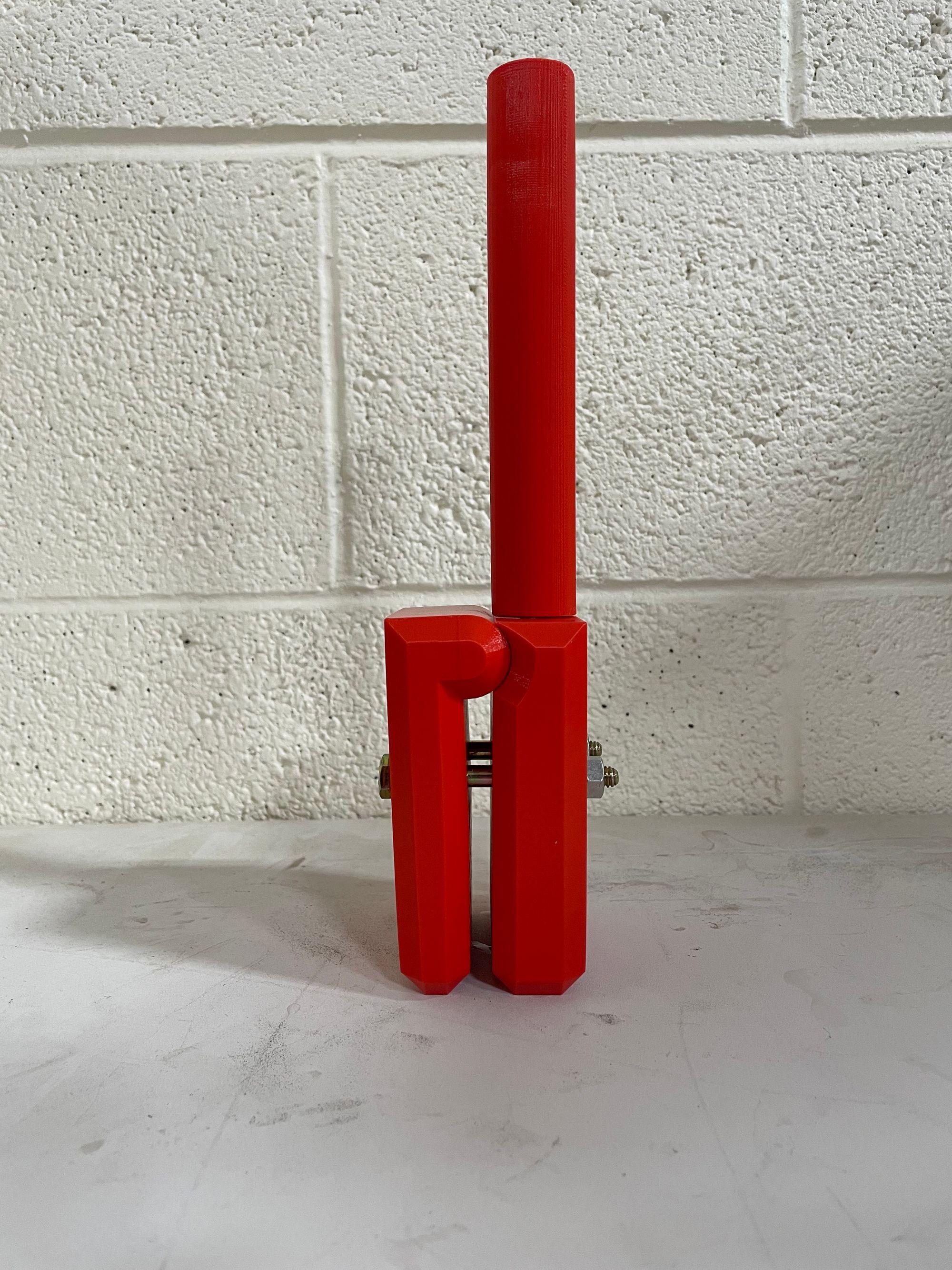
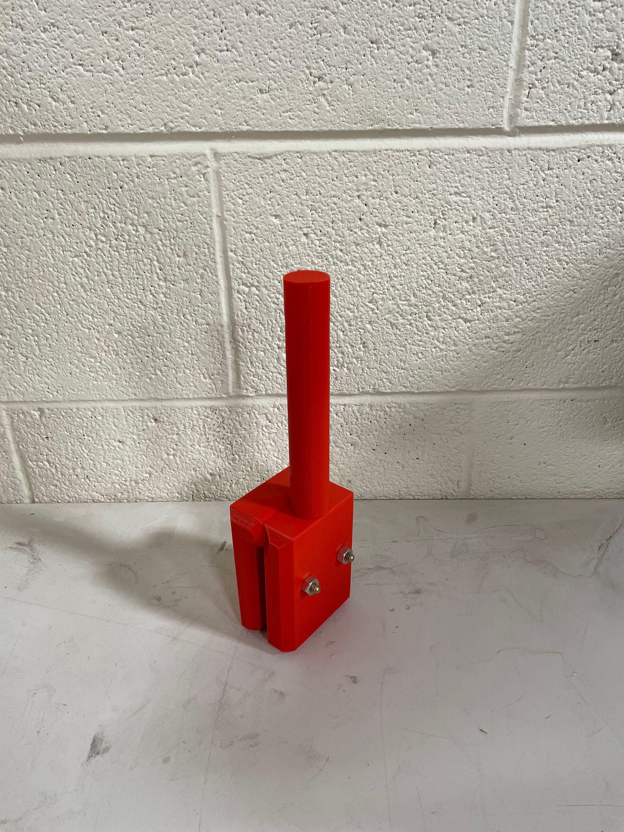
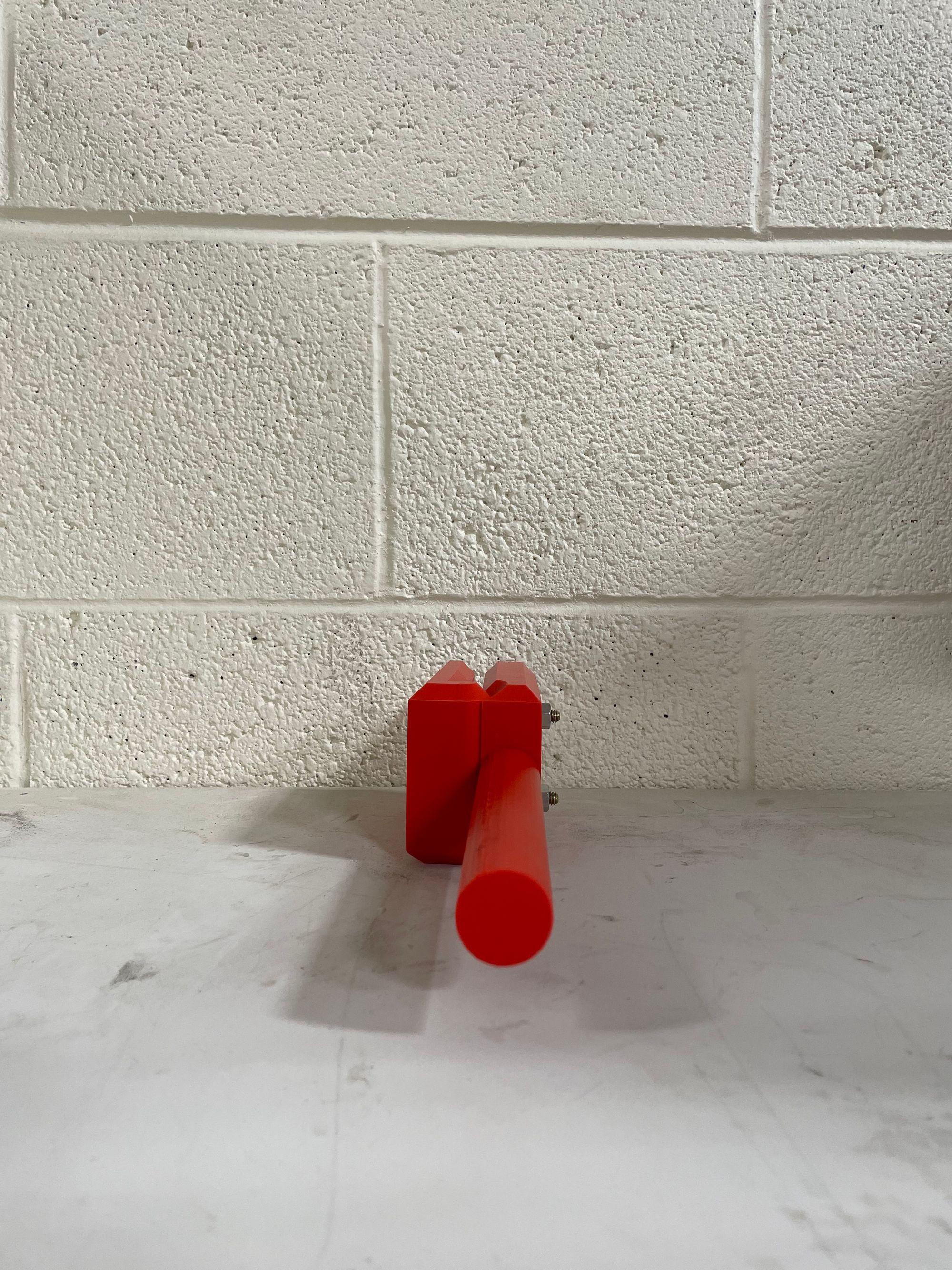
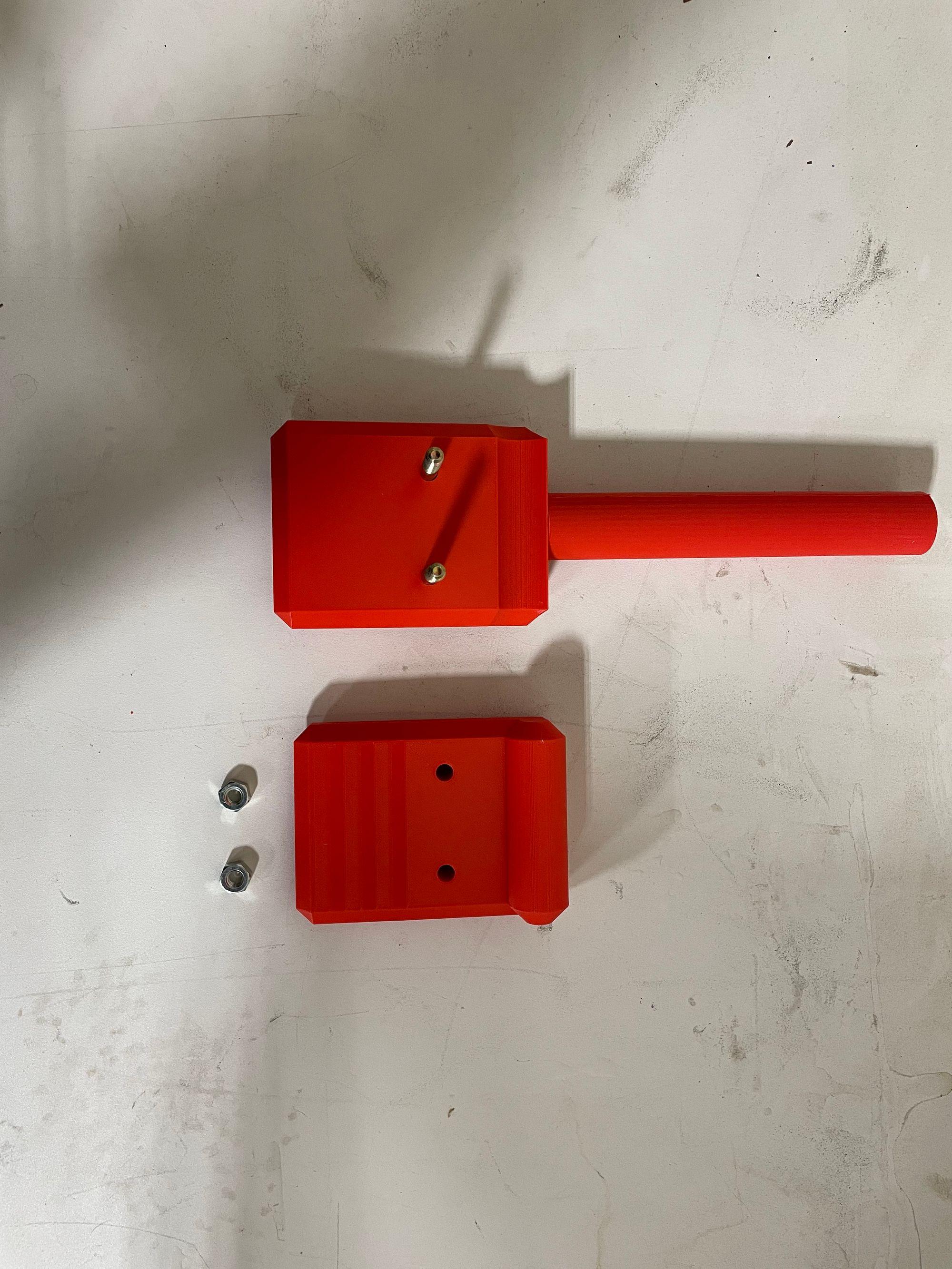
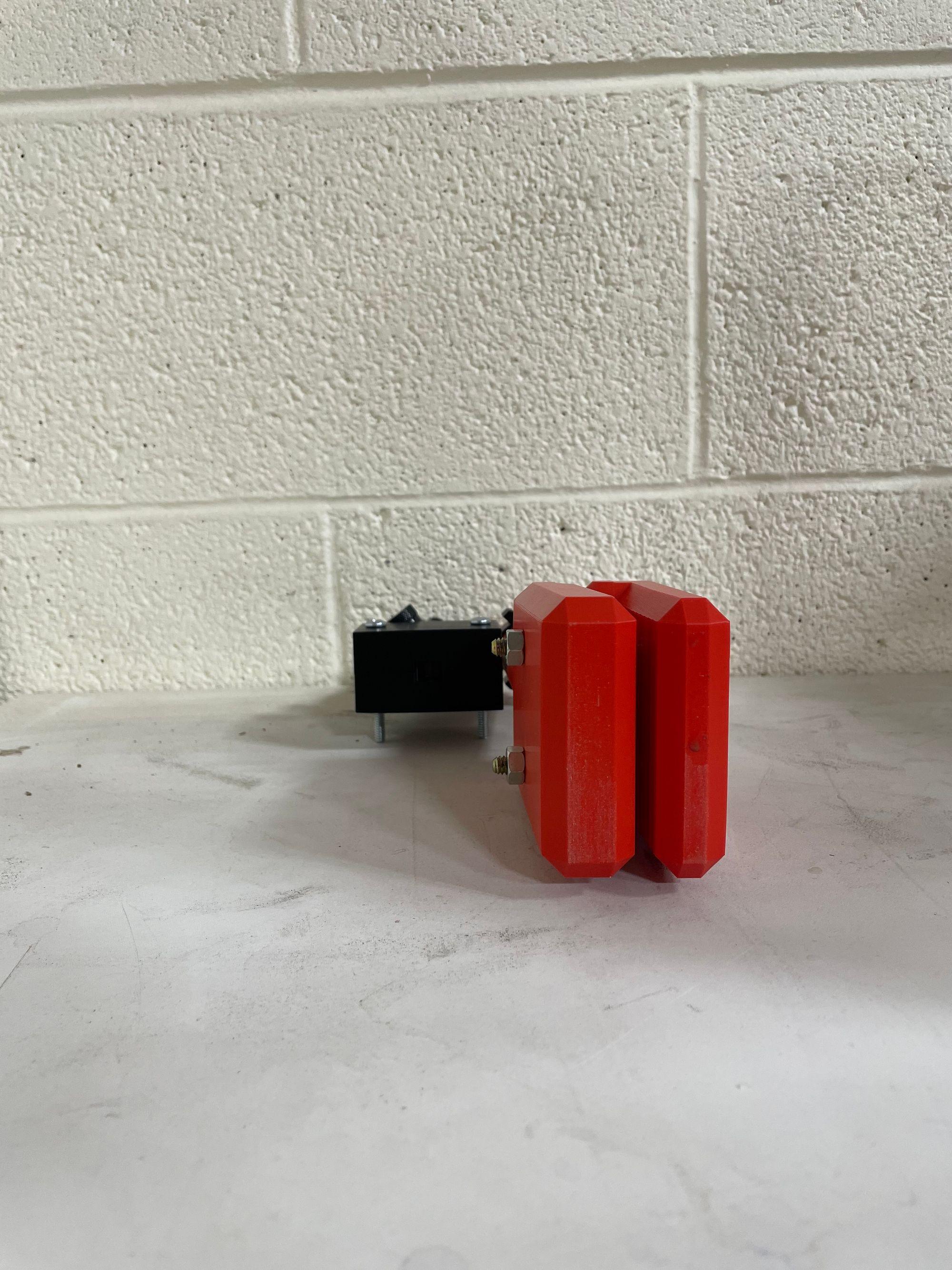
Assemble Laser/Lens Mount
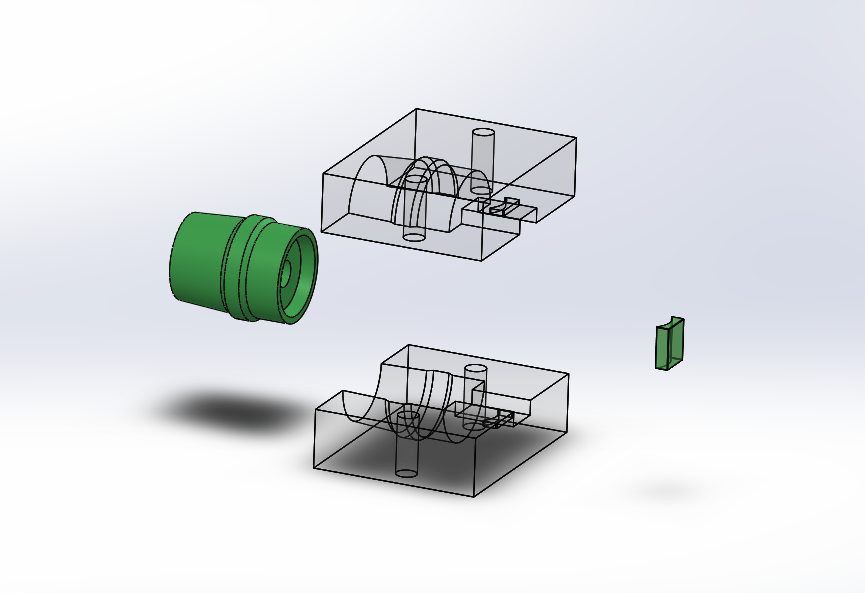
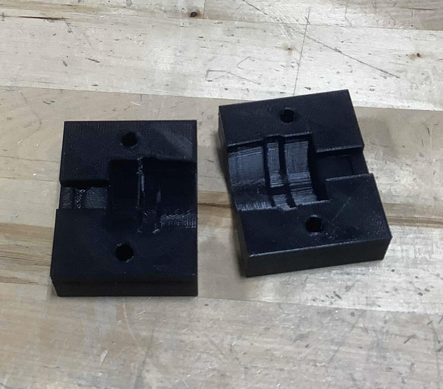
Assembly Instructions
- Adjust 3D printer settings if necessary and print two halves of the mount.
- Wash your hands thoroughly and place the lens in the lens-shaped indent on one half of the mount.
- Hold the front of the laser in place in the laser-shaped indent on the same half of the mount.
- Place the other half on top, making sure that the lens sits properly in place and that the top half is level.
- Use M6 screws (length 40mm or longer) to clamp the two halves together, making sure that the clamp is not pressing down on the lens with too much force.
- Adjust the knobs on the laser to ensure that the beam is centered on the lens.
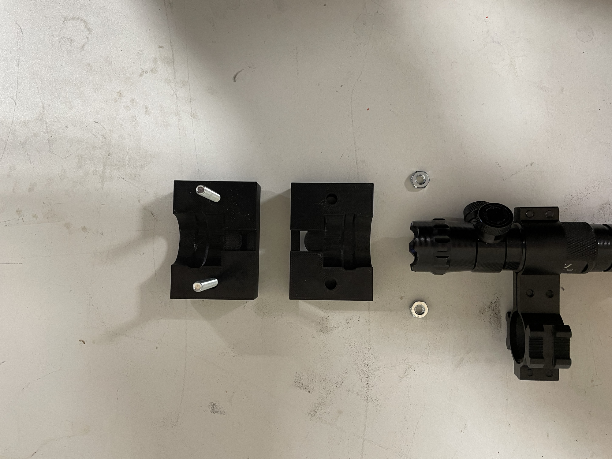
Assemble Tank Clamp
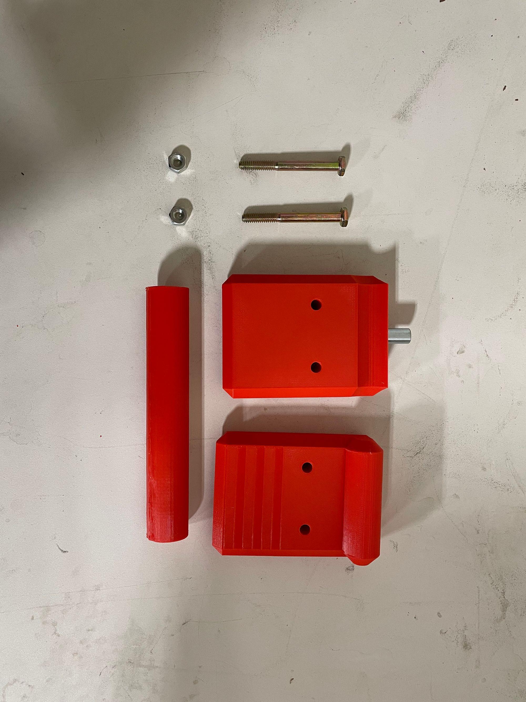
Assembly Instructions
- Adjust 3D printer settings if necessary and print two halves of the clamp and the rod.
- Remove bridging supports.
- Insert 1.5 inch cylindrical rod connector (not 3D printed, just hardware) in side 1 and the rod to connect the two 3D printed parts. You may need hot glue to secure these pieces together.
- Use 1/4-20, 4 inch long screws to connect the two halves, making sure the rounded pieces fit together.
- Attach to the side of the tank and fit laser attachment over the rod!
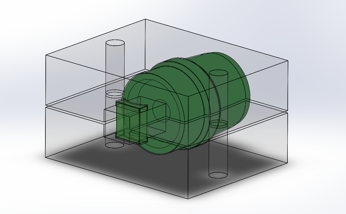
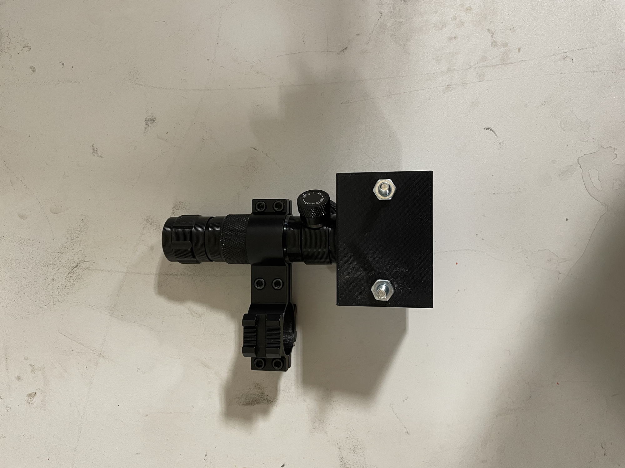
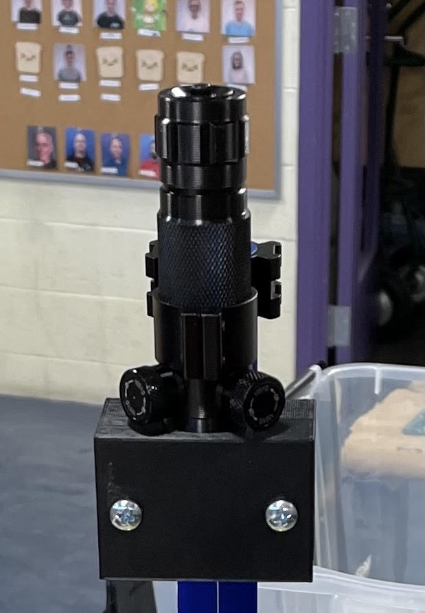
Create Final Assembly
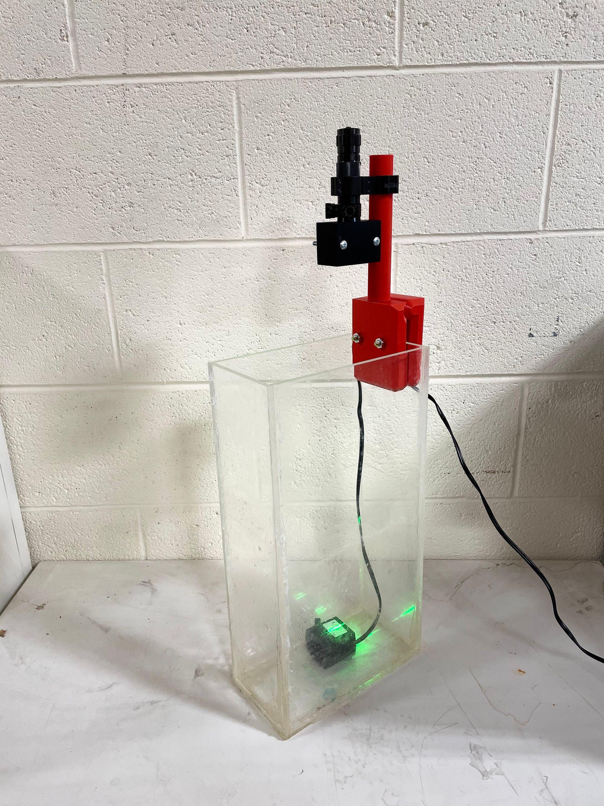
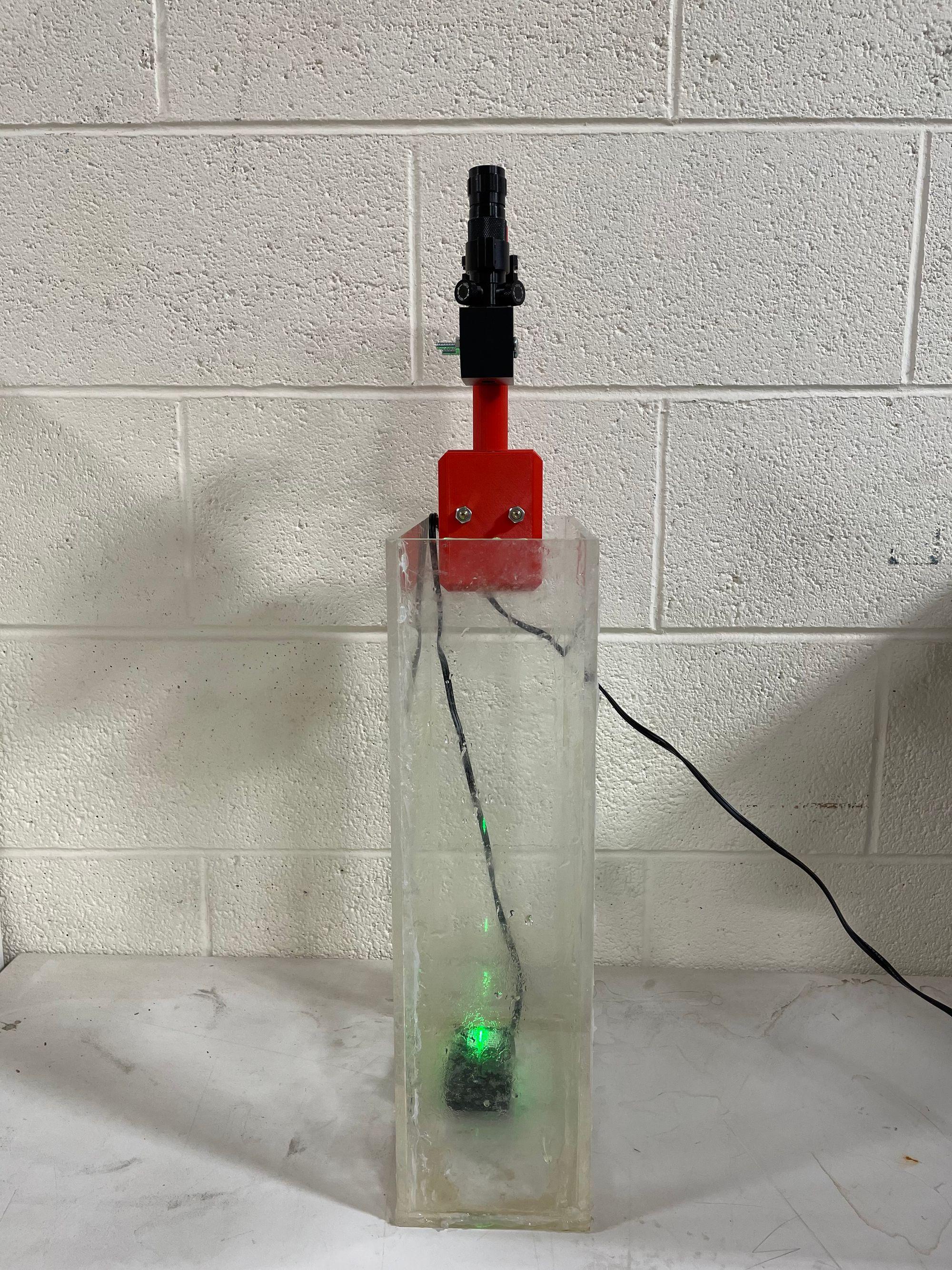
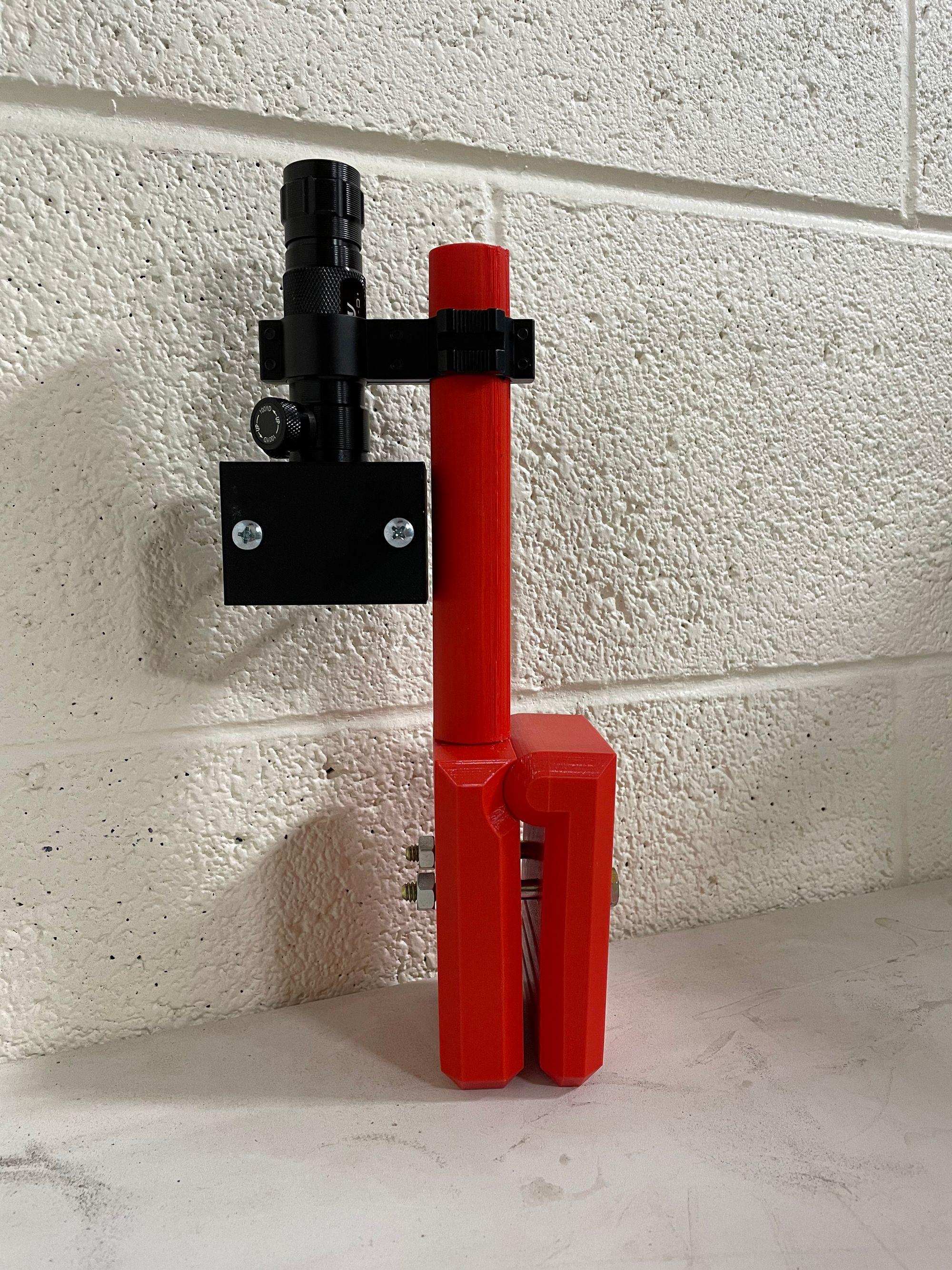
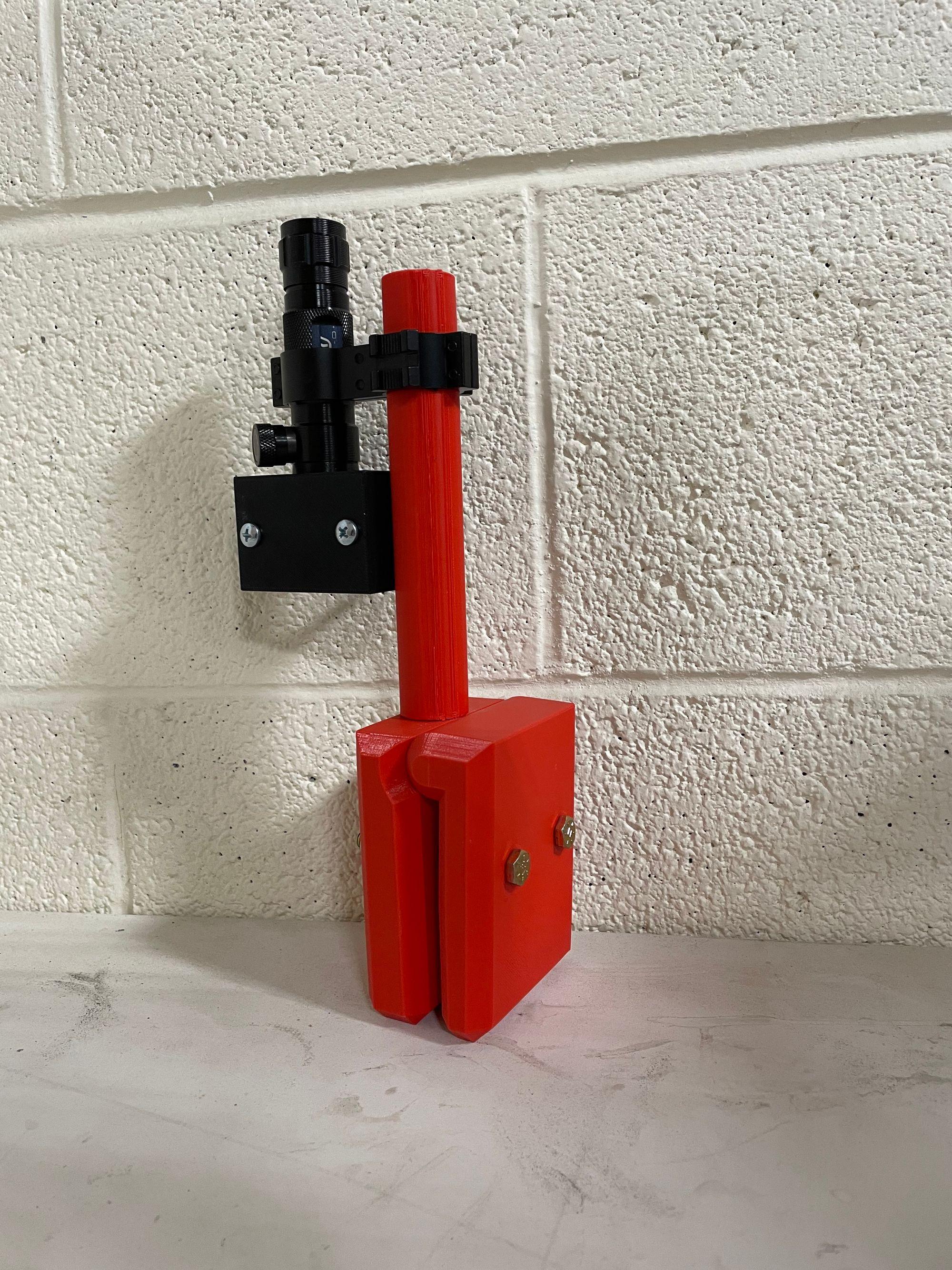
Connect the mount and clamp as shown.
Experimental Testing
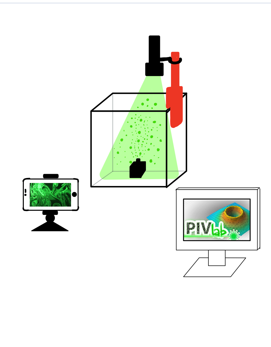
The laser-lens mounting system can be used on flow systems of all sizes. The system can be tested it with different pump speeds and flow rates as well. In this testing plan, we will analyze one particular flow set-up of the low-cost PIV, using the materials outlined above.
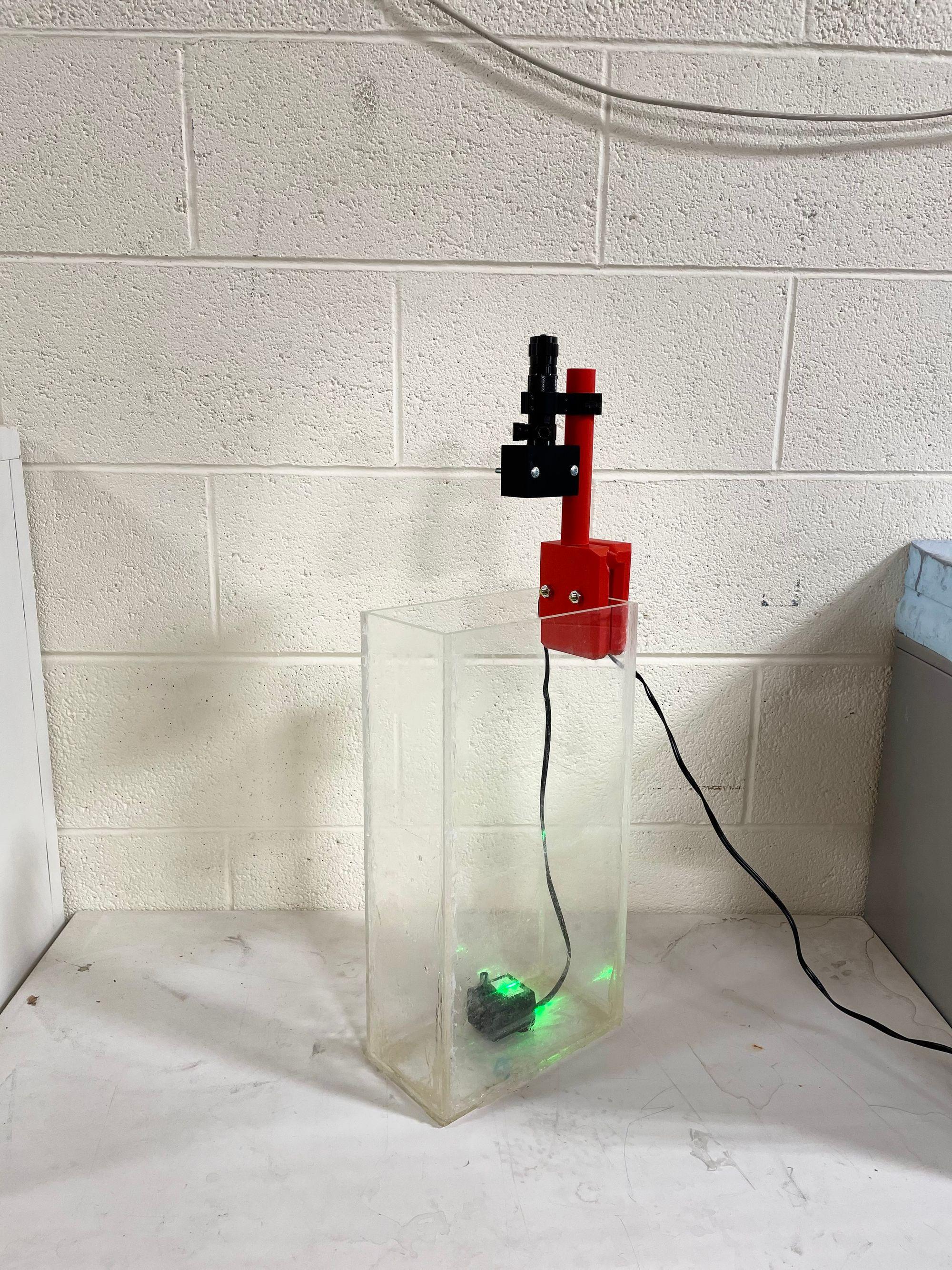
- Before beginning testing, wash the acrylic tank with water and dry with paper towels to ensure the walls are clean. Place the submersible water pump in the bottom of the acrylic tank. Fill with water, and a 1/4 teaspoon of seeding particles. Stir the water to evenly distribute the particles.
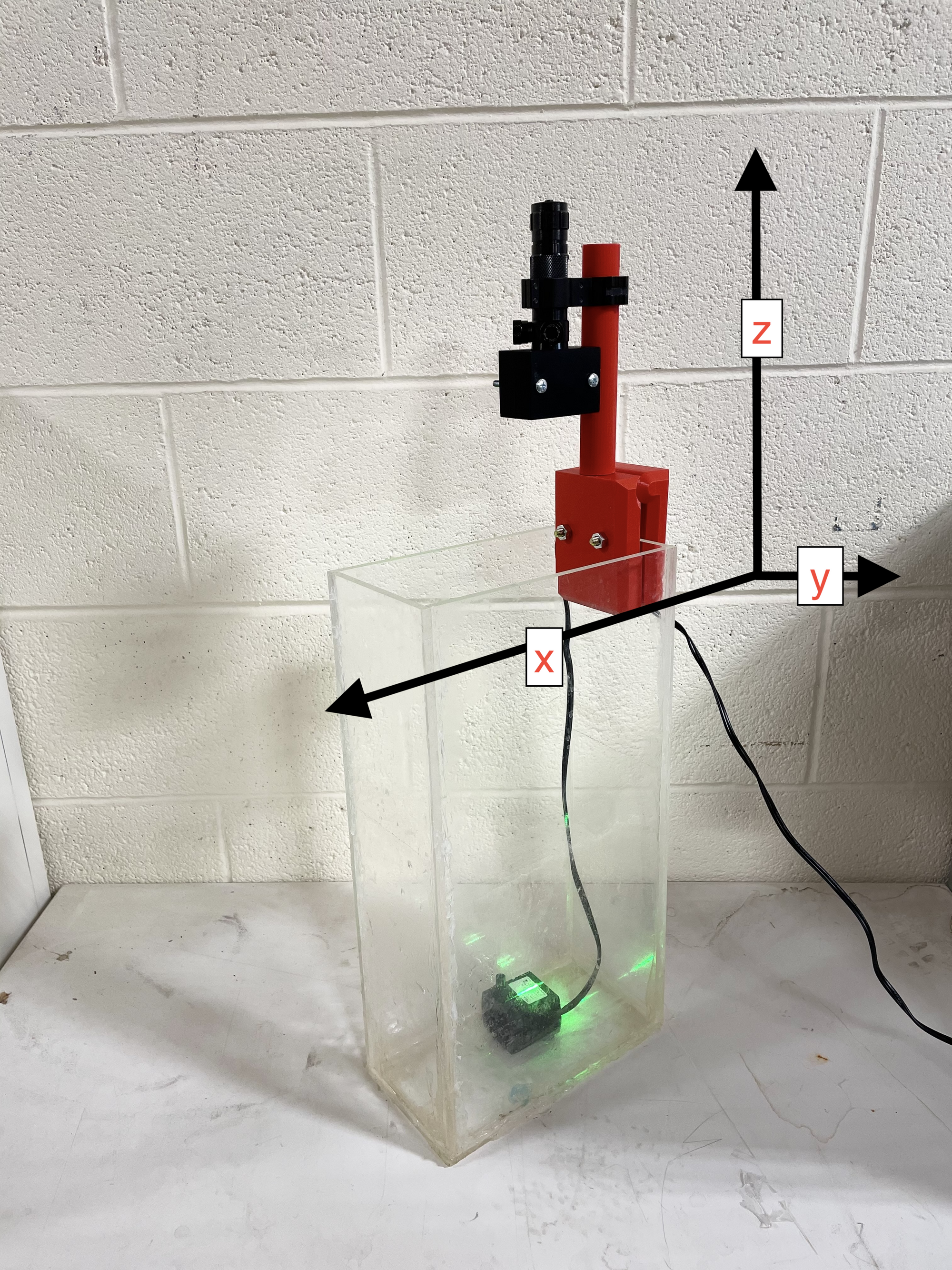
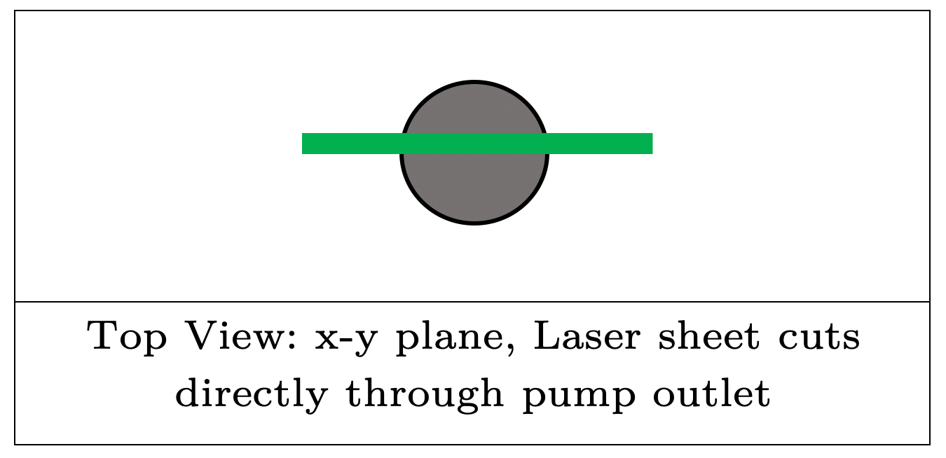
- Place the fully assembled laser mount system on the tank, such that the light sheet is directly over the pump’s outlet flow. The laser mount system is adjustable in the x-y, x-z, and y-z planes. Turn on the laser to ensure the laser sheet cuts directly across the pump flow.
- Securely attach phone camera to the phone stand, and place it in the direction such that it captures images in the y-z plane.
- Place the blank white construction paper behind the tank in the y-z plane, opposite the phone camera. This will ensure an even intensity background during software processing. In addition, turn off the lights to reduce glare and exposure during image processing.
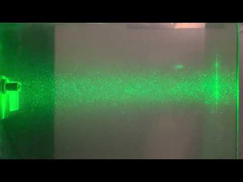
- Set the camera setting to 120 fps in slow-motion. Plug in the pump, and turn on the laser. Double check that the laser sheet has not shifted and is capturing the fluid flow.
- Focus the camera on the green lit seeding particles and capture a slow-motion video.
Download PIVLab/Image Processing Toolbox
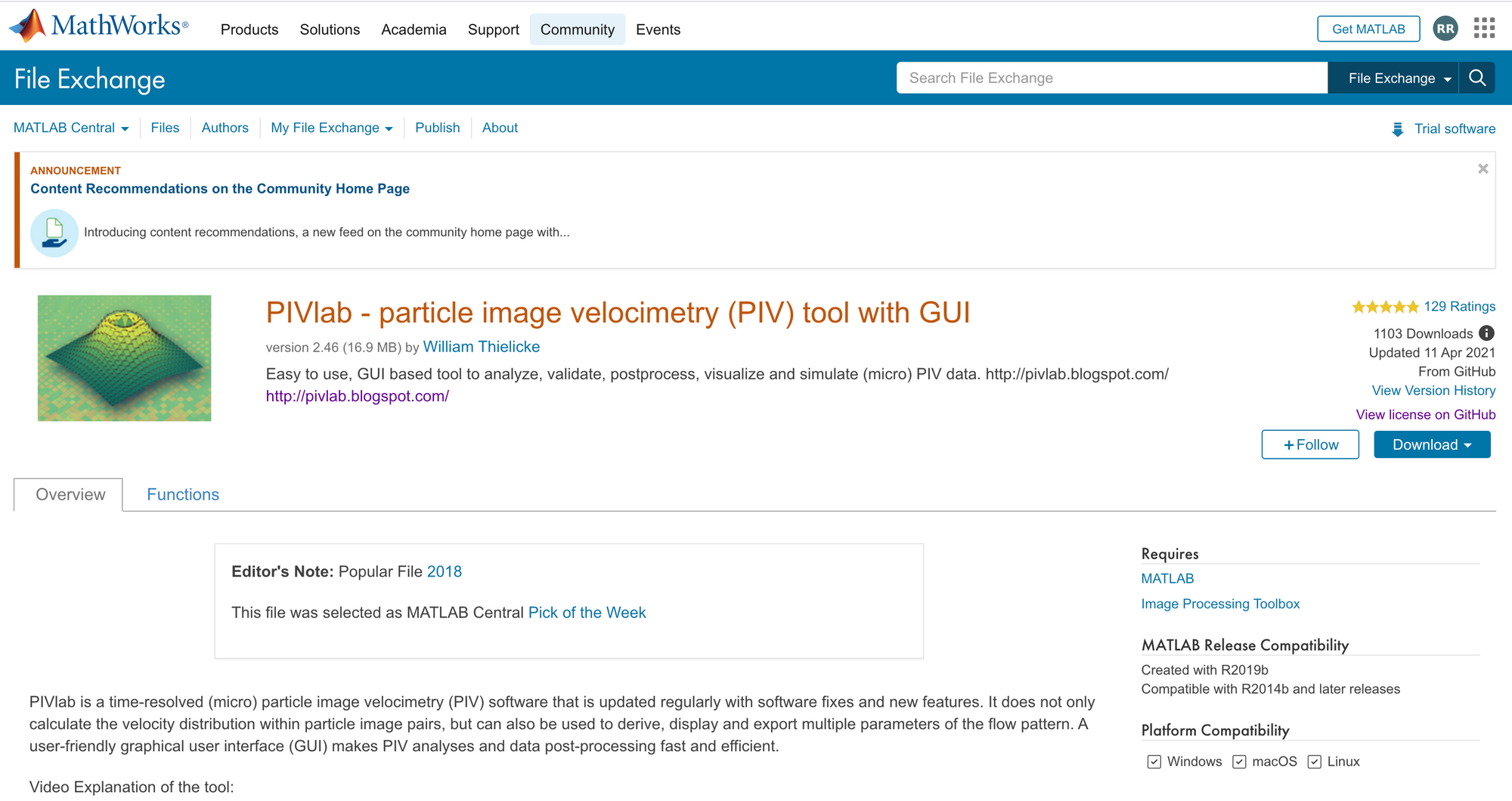
In order to analyze the images, you must download the image processing toolbox in MATLab, in addition to the PIVLab app. Simply visit MathWorks and download the image processing toolbox. To download PIVLab, visit here and download the toolbox. Make sure MATLAB is open and running on your desktop. Then download the toolbox, and the PIVLab app should appear within the MATLAB apps in the top toolbar.
Software Processing
Before opening PIVLab, access the preprocessing MATLAB scripts above.
A. Pre-Processing Video into Black and White Photos
- Upload the phone camera slow-motion video to your computer. Add your video to the same folder as the prepre.m script and make sure you fill in the correct video file name where it says to put it. This script creates a new folder, converts the video to image frames, and saves the image frames as black and white png images.
- Open the PIVlab GUI by running the PIVlab_GUI.m file, then select file, new session, load images, and select the range of images you’d like to analyze. Select Add, Import, then ok.
- For pre-processing inside PIVlab, we noticed that our images did not have a lot of dark values, rather they had many middle-toned greys. For this reason, we chose to select ‘subtract mean intensity’. We also selected ‘enable CLAHE’ and ‘enable highpass’ because these settings give our image the highest contrast and resolution for our particles.
- Set up exclusion zones, masks, and regions of interest (ROI) to focus on specific parts of the image. In particular, apply a mask where your pump outlet is in the frame.
B. PIV Settings and analysis
Once PIVLab is installed, it should pop up as an app in the top bar. Open PIVLab and click load images. Make sure your file path is the same as the location of the black and white photos. Select Time Resolved under Image sequencing Style ([A+B], [B+C], [C+D]…) for cross correlation. Click Browse, and select the consecutive preprocessed black and white photos of the flow. Click Add, then Import. One image should be largely present on the screen.
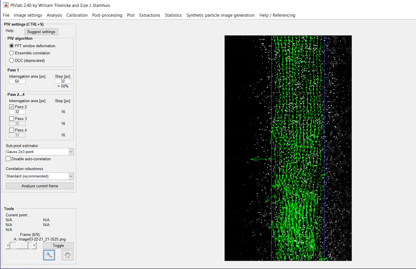
In the top bar, right click Image Settings, then select Exclusions (ROI, mask). Select a region of interest by dragging your mouse over the image. Apply the window to all frames. Create an object mask over the pump. To further improve image settings, right click image, then select Image Pro-Processing. Tick the first three boxes to improve image quality. Next, go to Analysis in the top bar, and click PIV settings. Use the FFT algorithm. Make sure Pass 2, 3, and 4 are set to 64, 32, and 32 respectively. Analyze all frames. You will hear the voice, PIVLab finished.
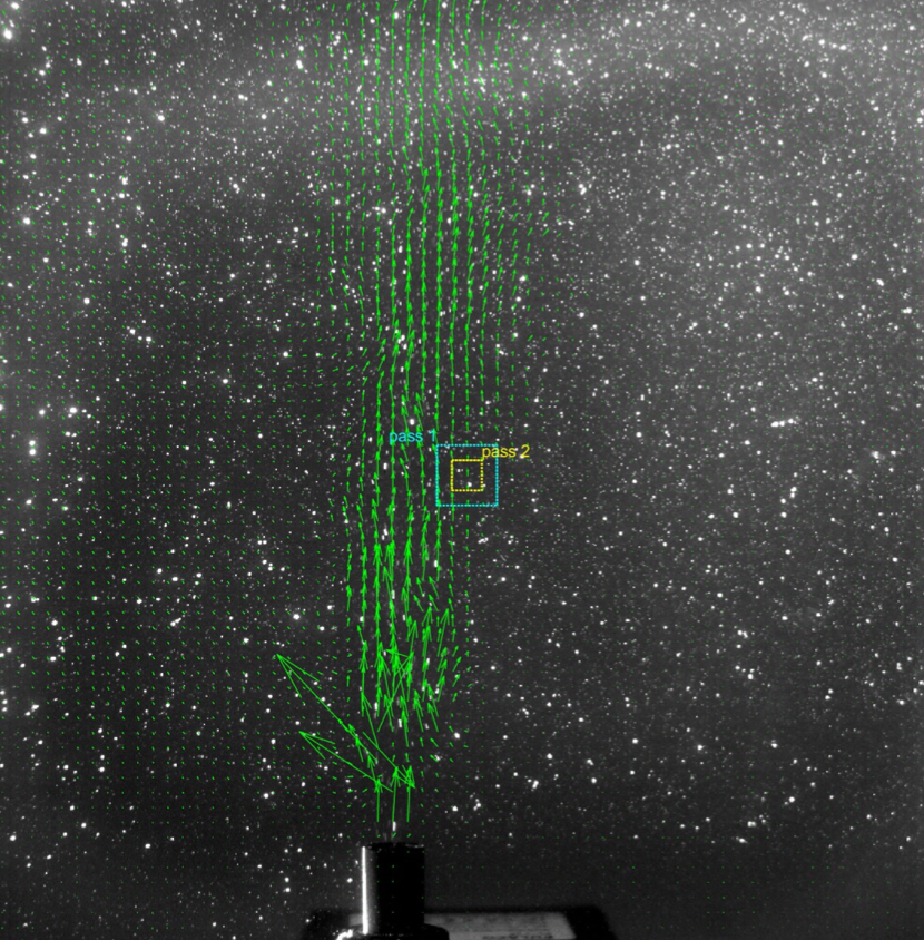
It is important to pause and qualitatively analyze the velocity field results. If an arrow jumps far from its tail, and overlaps other arrows, this means the flow rate is too large for the frame rate to capture. If this occurs near the pump outlet, that is not a large concern. However, if this problem is present at all locations on the vector field, it may be important to repeat the experimental procedure with a slower pump flow rate.
C. Post-Processing
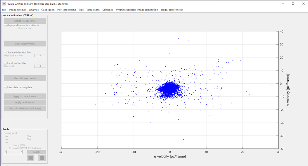
Go to the post processing tab and select vector validation. You’ll want to narrow the bounds of the vectors shown so that all vectors show physical results. If one part of the stream was too fast for the frame rate or for the window size, you’ll have to manually reject the vectors in that area by forcing all velocities to have a min and max. Draw that min and man area using a rectangle on the blue dot plot above.
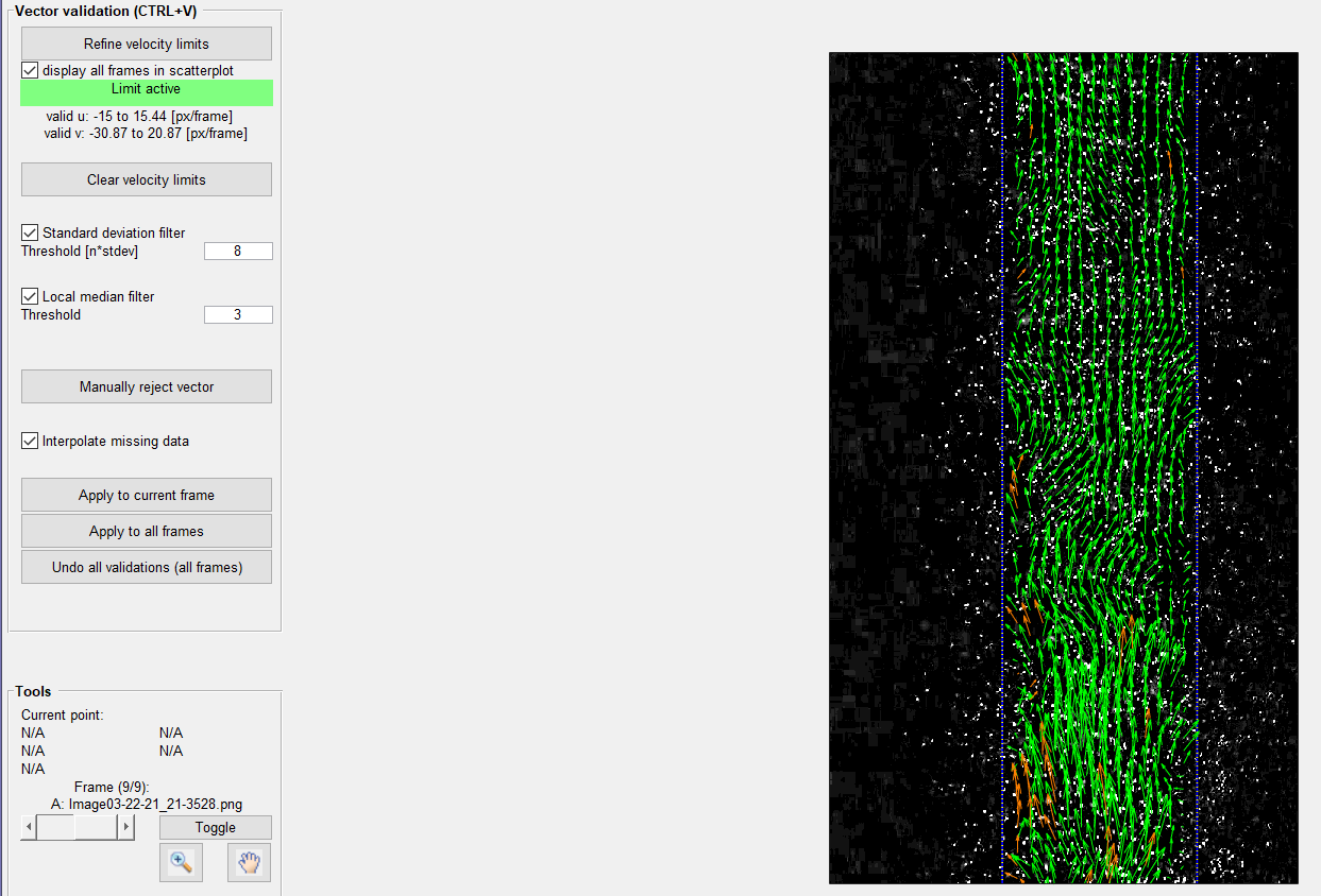
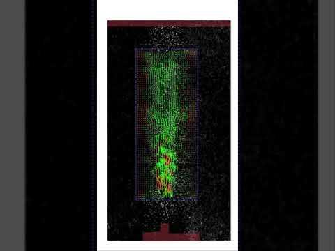
Under Post processing in the top bar, select Vector Validation. Click refine velocity limits, and drag and select a window of concentrated velocities disregarding outliers, shown above. Apply the limits to all frames. This will generate velocity fields, such as the one shown below. Under Plot in the top bar, there are many different functions, such as vorticity, to select and graph, depending on user needs. Play around with those functions to the user's desire.
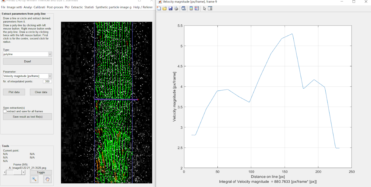
D. Generating Data
To gather velocity data over a cross-section of the flow, go to Extractions, Parameters from polyline. Then draw a line, shown below in pink, and select the parameters you want to examine. The plot of distance vs. velocity is created when you select Plot Data. The velocity is measured in px/frame.