Intro to Excel: Expense Tracker
by watchmeflyy in Circuits > Microsoft
22213 Views, 219 Favorites, 0 Comments
Intro to Excel: Expense Tracker
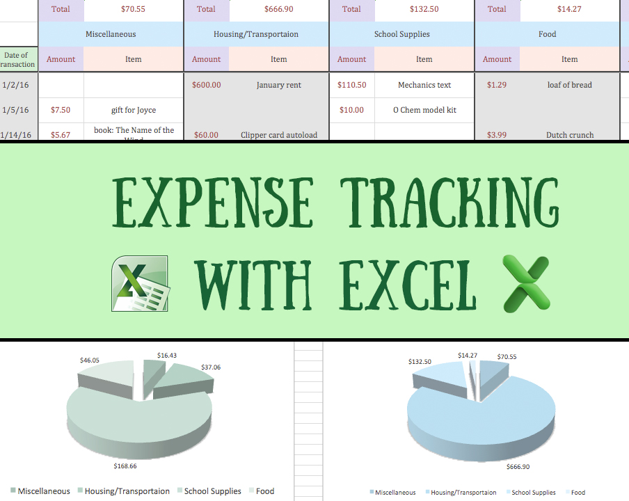
I like to record my monthly spending patterns to get a good feel for how much I'm spending in certain categories, whether I'm going in monthly deficits, etc. I've been updating a custom Microsoft Excel (the spreadsheet program of the Microsoft suite) spreadsheet for this purpose, and one day a friend saw it and asked me to teach her how to make something similar. Even my brother has asked me to send him a template, so I thought this tutorial might come in handy for others too.
I'll essentially be going over basic Microsoft Excel functions and tips as this tutorial progresses, so no need to worry if you've barely opened a spreadsheet before. But learning how to make and maintain spreadsheets is a valuable skill that can save you time, paper, and brain power (Banking check books work fine, sure, but online copies are quite convenient once you get the hang of it!). Even if you're an excel wizard, perhaps you'll still find step 10 helpful (I'm fairly proud of the notes I took while I read up on how to use Excel...).
Side notes: votes in contests would be very much appreciated if you like this tutorial. :)
Spreadsheet Programs
Excel is the well-known spreadsheet application out there, but there are nice, free alternatives also for those who don't have access to the MS suite. I've heard good reviews about KingSoft, for example. MacBooks come with an application called Numbers in its iWork suite that also handles spreadsheets, but honestly I've never tried it so can't provide feedback on that.
Google sheets is one I can recommend: it's very convenient in that it saves your file in your Google account so that you can access it from any computer/smartphone/tablet with internet access.
Bottom line: don't fret if you don't have Excel! Work with what you have, and you should be fine. My tutorial uses Excel, but most programs if not all have some equivalent to the functions and controls I'll be using, though in different toolbars or menus. Also, side note, I am fortunate enough to have a Mac but Windows/Linux/etc. users will need to figure out the locations of the buttons I reference.
Free Templates
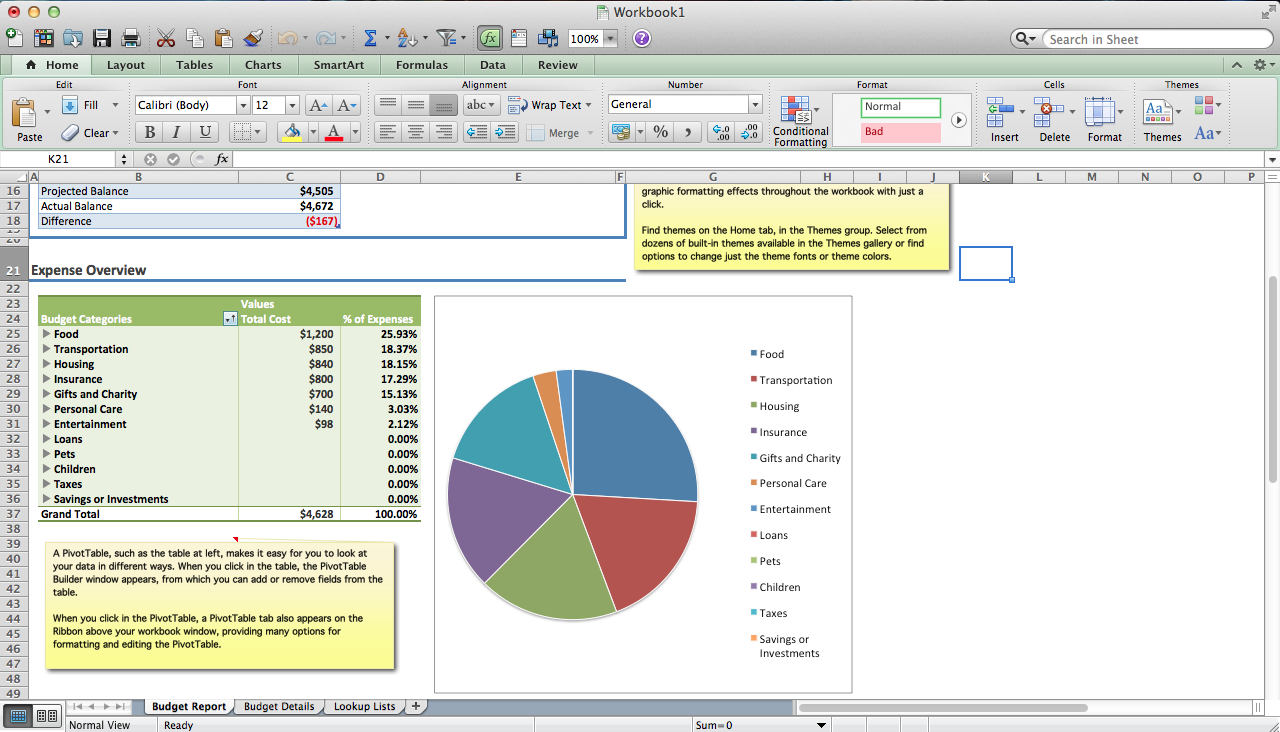
Excel and many other programs provide pre-made templates for easy use. In fact, you can find some online as free downloads.
However, I find most of them a bit too complex for what I need. For example, if you look at the screenshot above of Excel's expense tracker, you can see columns for charity, pets, loans, taxes, children, etc. -- very comprehensive, yes, but not necessary for my mundane purposes. Plus, making my own template gave me a comprehensive view of the functions my sheet has, rather than playing around and altering a pre-made sheet. And mine suits my aesthetic tastes better *sticks nose in air*.
The decision is up to you though: ready template or custom.
Tutorial Overview
Is this tutorial unnecessarily long? Perhaps. I just want to be as comprehensive and clear as possible.
Anyway, an overview: the next couple steps introduce the Excel interface and basic commands that come up in working with spreadsheets. No, I won't cover every little detail, but I'll explain as much as any beginner should know for handling Excel. After that, the rest of the tutorial goes into how to actually create the expense tracker (disclaimer: it will be in my tastes/preferences but you can alter as you see fit, using commands/tools I'll explain along the way), ending with additional resources and applications.
Opening a File
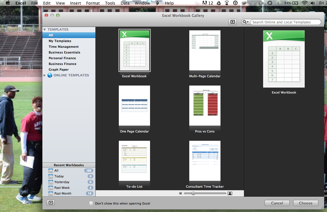
Now with the tutorial: (side note: pictures are provided if you can't find what I'm talking about in the text)
Start up the Excel application and open up a new file. A new window might just pop up from starting the application, if that was a pre-set function on your computer, or you can manually go to file (at the top menu bar) and clicking "New Workbook" (yes,
these spreadsheets are called workbooks. Alternatively, you should see the list of templates in a small window: double click the Excel Workbook option (or any other option, once you want to play around with other possibilities). OR you can do the keyboard shortcut ctrl/command + n to automatically open a new file.
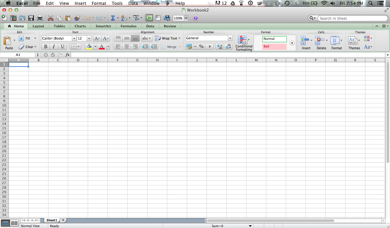
In any case, you should end up with some opened spreadsheet.
Top Toolbar

At the top of the workbook, you should see a row of buttons with various functions (you might not have the exact same depending on version, customization, etc.).
These include:
- open
- paste
- save
- cut
- copy
- copy format
- undo/redo
- statistic commands
- arrangement
- filter
- zoom
- help
among other functions. See the picture above for more details and how they work.
Tabs: Home

Below that top toolbar should be a system of tabs: home, layout, tables, etc.
In the Home tab, you can see several useful functions, among which are:
- paste
- fill
- clear
- font customization
- alignment
- wrap text
- number formatting
- conditional formatting
- cell formatting
among other functions. See the picture above for more details and how they work.
Tabs: Layout

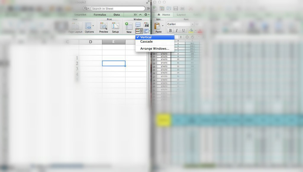
In the Layout tab, you can see a few useful functions (not as many as home, but still useful), among which are:
- general page formatting
- freeze rows/columns
- arrange windows
among other functions. See the picture above for more details and how they work.
Tabs: Tables

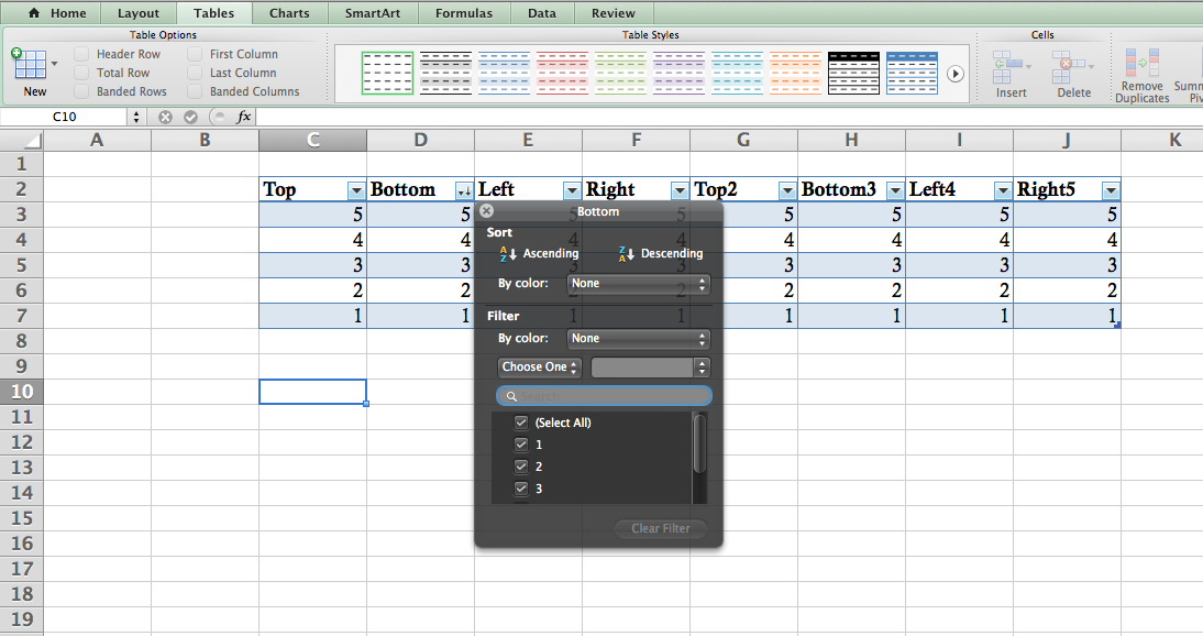
In the Tables tab, you can see a few useful functions (not as many as home again, but still useful), among which are:
- table formatting
- removing duplicates
- adding/removing cells
among other functions. See the picture above for more details and how they work.
Tabs: Charts

In the Charts tab, you can see a few useful functions (not as many as home again, but still useful), among which are:
- chart types
- chart styles
- chart formatting
among other functions. More tabs pop up once you actually make a graph, but I'll cover that later. See the picture above for more details and how they work.
Yes, there are a few more tabs (SmartArt, Formulas, Data, Review) but I haven't used them enough to provide much detail. Look them up if you'd like, and consult guides (see last step of this tutorial) -- sorry!
Function Bar, Row/column
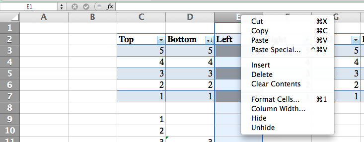
Below those tabs you have your workspace and the sliver of space to type in functions over it. The function bar allows you to type in the cell's value (eg. click on A2 and type "2" to assign it a value of 2). You can also type in actual functions, such as " = B2 - T6 " for a cell.
Control rows/columns by highlighting them for selection, right clicking for pasting or sizing options, or dragging for changing their width manually.
Little Shortcuts
I've also compiled a short list of little tips and keyboard shortcuts for ease of use:
- Pressing shift + an arrow key (up/down/left/right) will advance your selection be as many cells as you press for the arrow key (press up twice to select two more cells up, etc.)
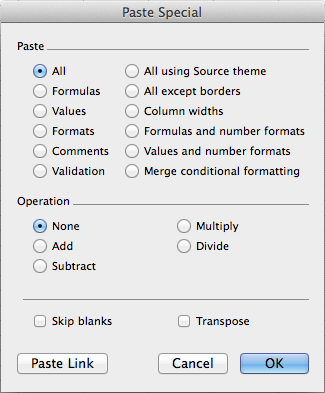
- Go to edit (on the top menu bar) > paste special (or right click for this option) to customize what you want to paste. This gives you better control, such as only the formatting or the plain text rather than the function.(see first picture)
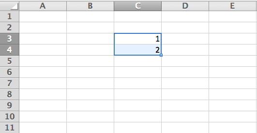
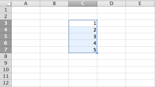
- Autofill cells by typing out enough to define a pattern (eg. 1 in one cell , 2 in adjacent cell on the right or below) and dragging the bottom right corner once you see the black cross icon for your mouse (see second picture).
- If you don't want a particular cell to change as you autofill, add a dollar sign in front of its coordinates. For example, I want to subtract cell A2 from a whole column so I type " = B1 - $A$2 " into B1 and drag the lower right corner to do that for the column of B. A2 will always be the one subtracted. If I leave out the dollar sign, it'll do B1 - A1, B2 - A2, etc.
- Track changes in your document (very useful if you shared it with someone else for editing) going to tools > track changes > highlight changes (can reject or accept them too)
- Minor trick = to stop the shimmering around a selected cell, press esc (selection is still loaded).
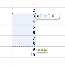
- Use a colon to select a range of cells. (third picture)
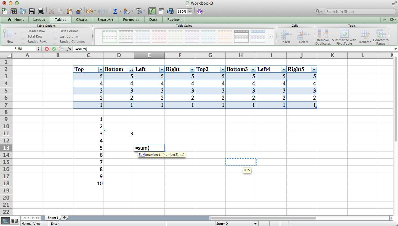
- Easily find out the sum, counts, mean, max, etc. of selected cells by clicking on the small box at the bottom of the workbook close to the middle. (fourth picture)
- Finding commands:
- type a?b to find acb, adb, etc. (any additional letter between a and b)
- type a*b to find asub, anananab, etc. (any additional number of letter between a and b)
- type ac~? to find EXACTLY ac?
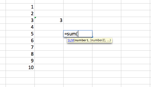
- Excel functions: Excel has some built-in functions that automatically sum, count, etc. for the cells you've highlighted. There are specific specialized ones for engineering or accounting too. Here are two links: one and two, but the ones I use the most are:
- SUM() sums up the cells you select in the parentheses
- AVERAGE() averages the cells you selected in the parentheses
- COUNTIF() counts up cells that meet a certain criteria
- Note: Excel is great in that it provides a small box to guide you on how to fill out the formula (the syntax of cell that go into the parentheses). (fifth picture)
Additionally, you may find some keyboard shortcuts handy:
- ctrl/command + n = opens a new blank workbook
- ctrl/command + p = open print dialogue window
- ctrl/command + s = save workbook
- ctrl/command + c = copies the cells you've selected
- ctrl/command + x = cuts the cells you've selected
- ctrl/command + z = undo the previous command
- ctrl/command + y = redo the previous command
- ctrl/command + f = find specific cells with keywords
- ctrl/command + h = hides window from screen (doing illegal business, eh?)
There are others, of course, but these are the ones I see as most useful.
NOW let's finally move onto the expense tracker, shall we?
Cell Size and Formatting
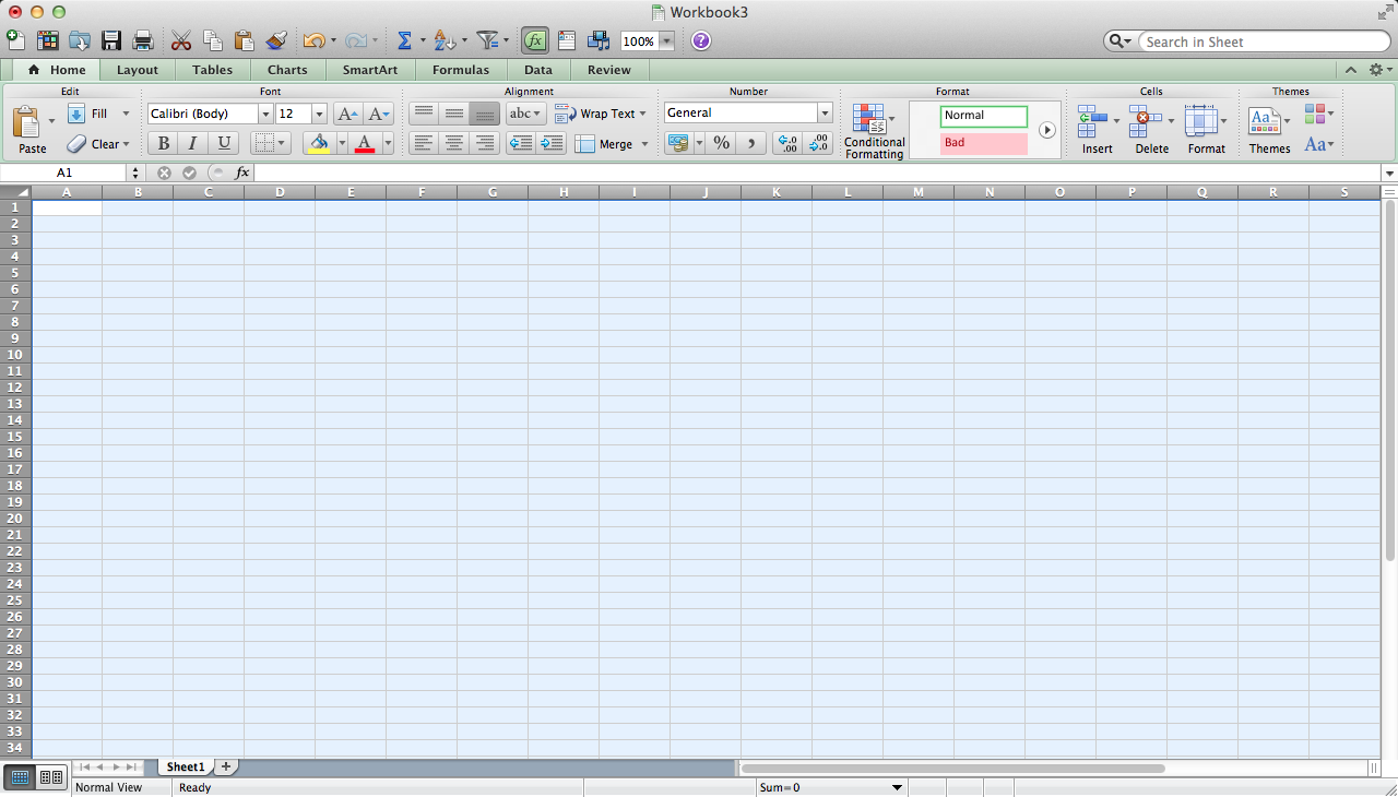
Open a file as shown in step 4.
To pre-format all your cells, you'll first need to select all of them. Click the arrow in the top left corner of the grid (see first picture) to select all cells, or press ctrl/command + a.
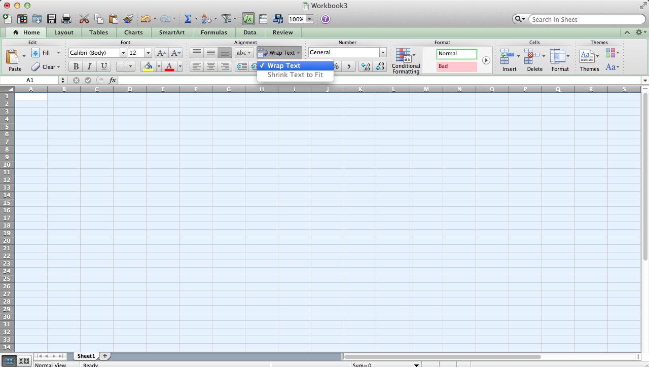
For the formatting, I like to make all cells' text wrap to another line if it's longer than the cell's width. To do so, click "wrap text" (second image).
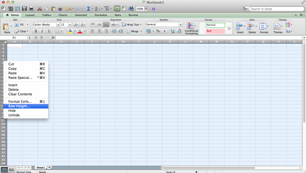
The cells are smaller than I'd like, so to change this I right click the rows on the far left and go down to "row height". 0.5" looks good to me; change as you like. Then click anywhere to stop the selection of all cells.
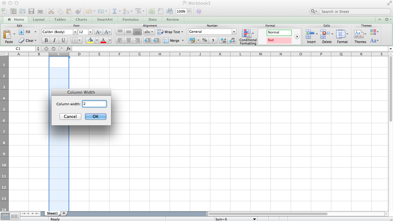
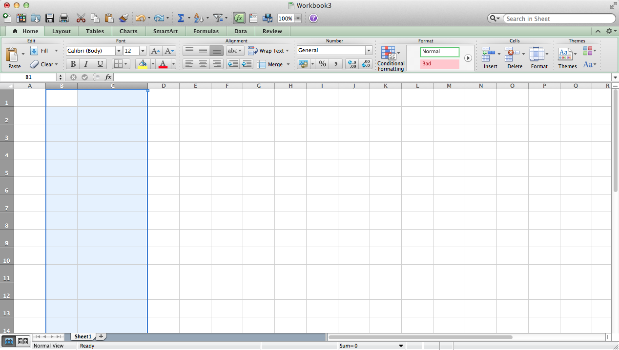
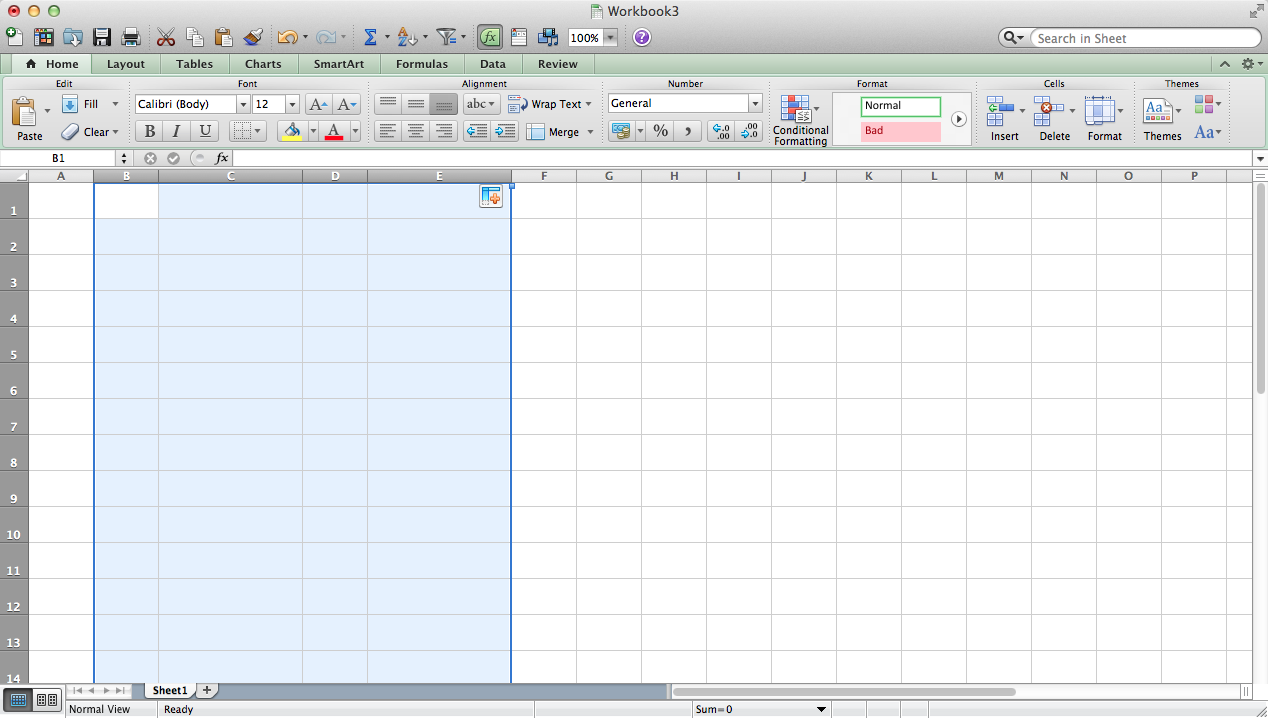
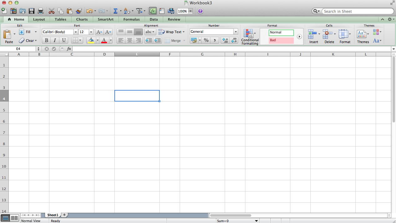
Don't ask questions yet and just do this for now (I'll explain later): select the entire column C by click the C at the top of the column before right clicking to set the width to 2". Then select BOTH C and B by holding down the shift key while clicking on the C and B columns. On the top right corner of column C, if you hover your mouse it should turn into a black cross. Click and drag with the black cross cursor so that D and E are selected before letting go. You should end up with something like in the fifth picture; B and C's formatting is copied to D and E's. I did this so that I could have a thin column for numbers and a wider column for explaining the transaction. Click and drag the formatting as before to cover at least until Z now, to make a uniform grid of similar columns.
You should end up with something like the last picture.
Labeling
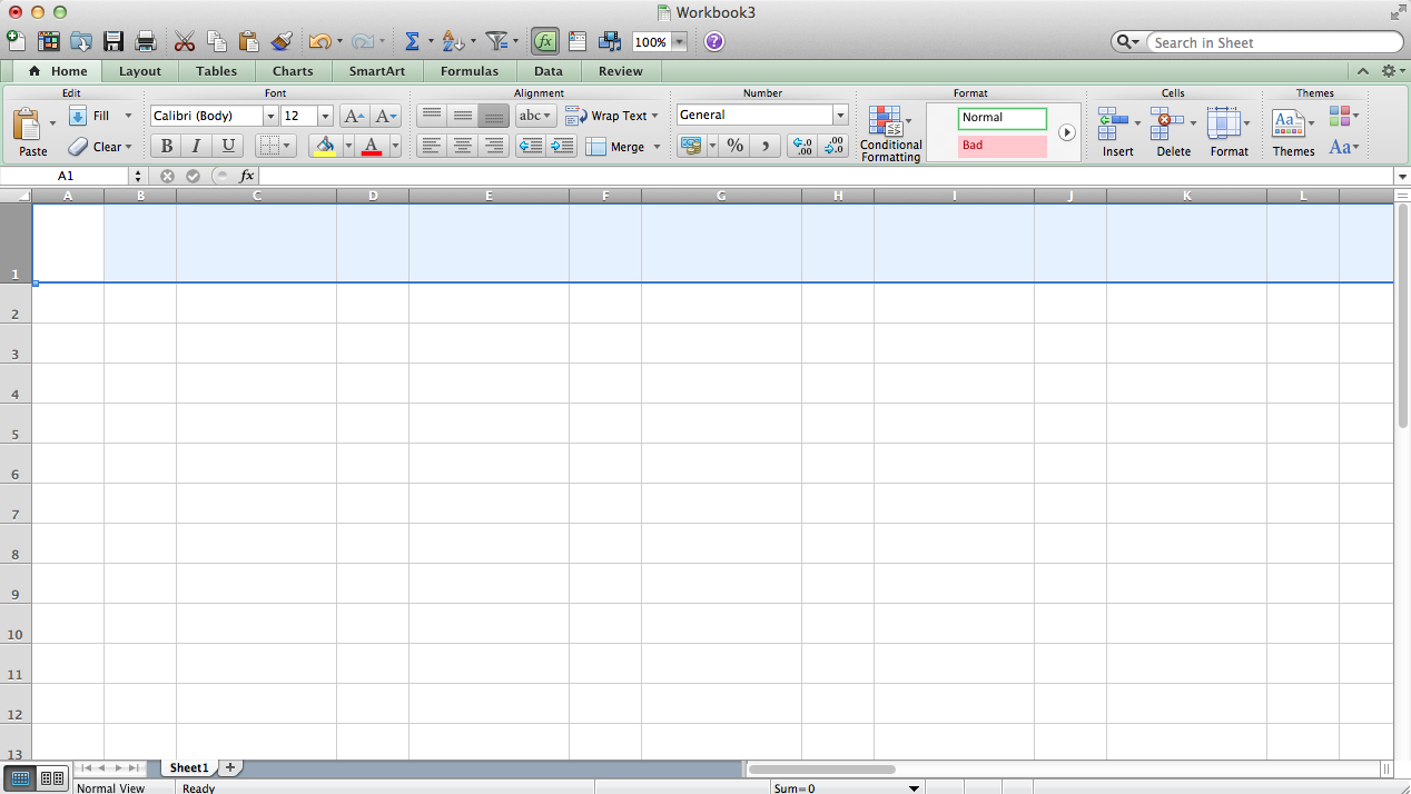
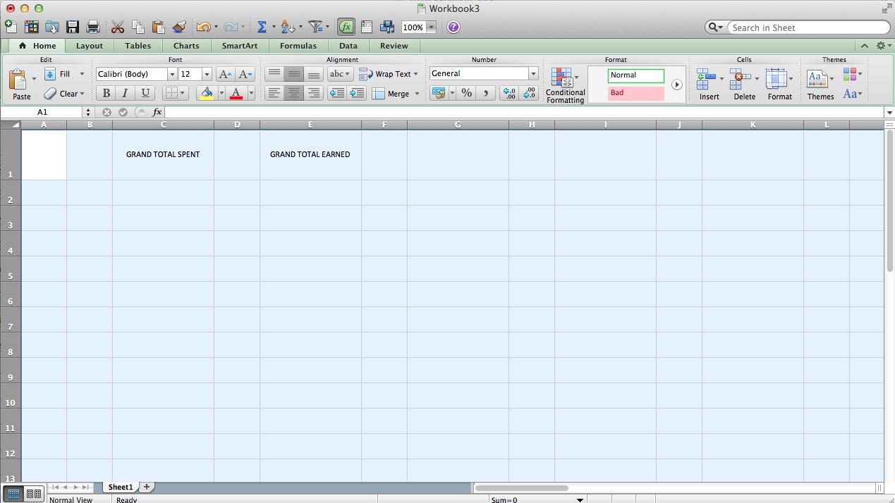
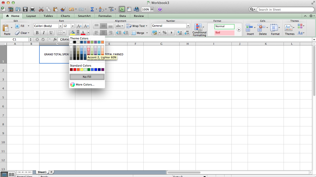
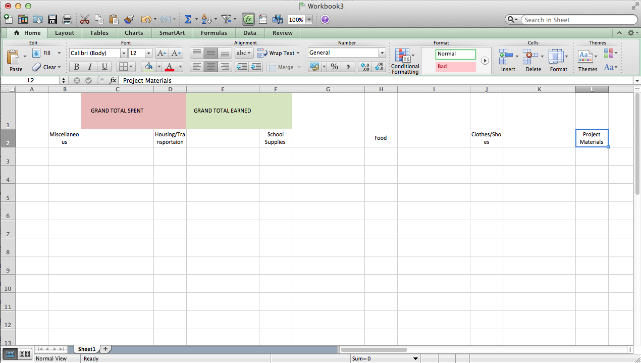
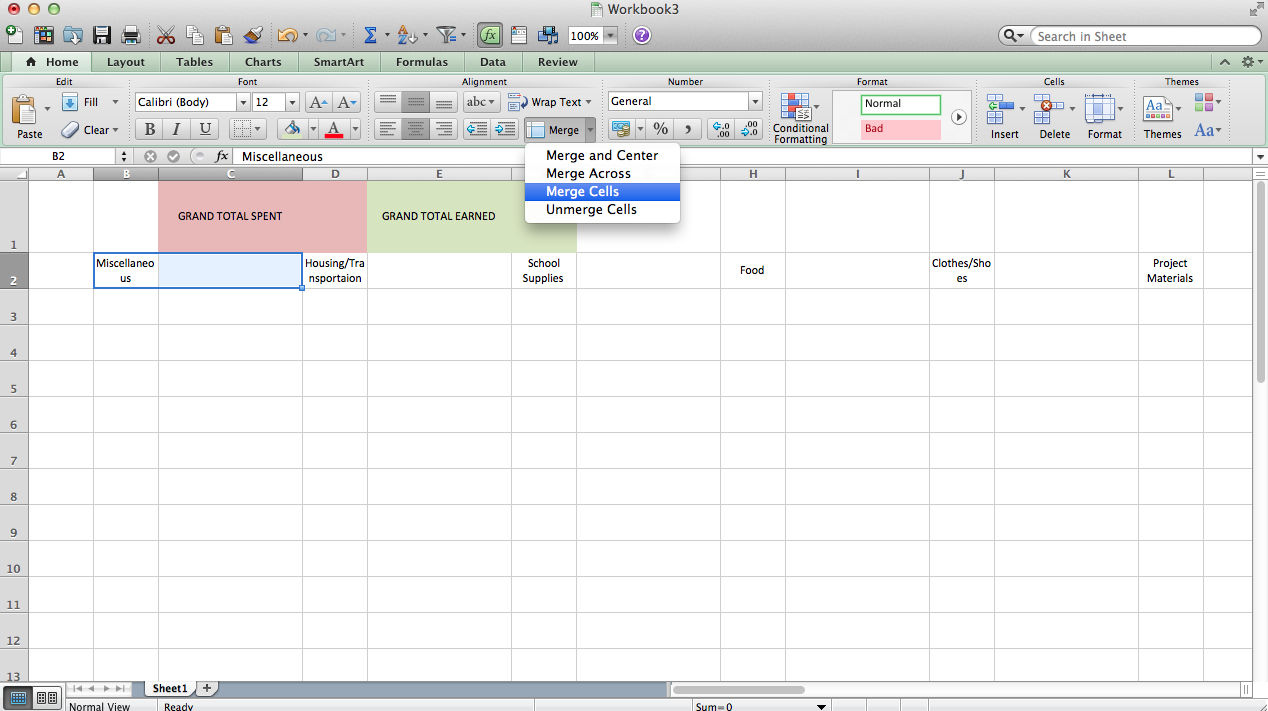
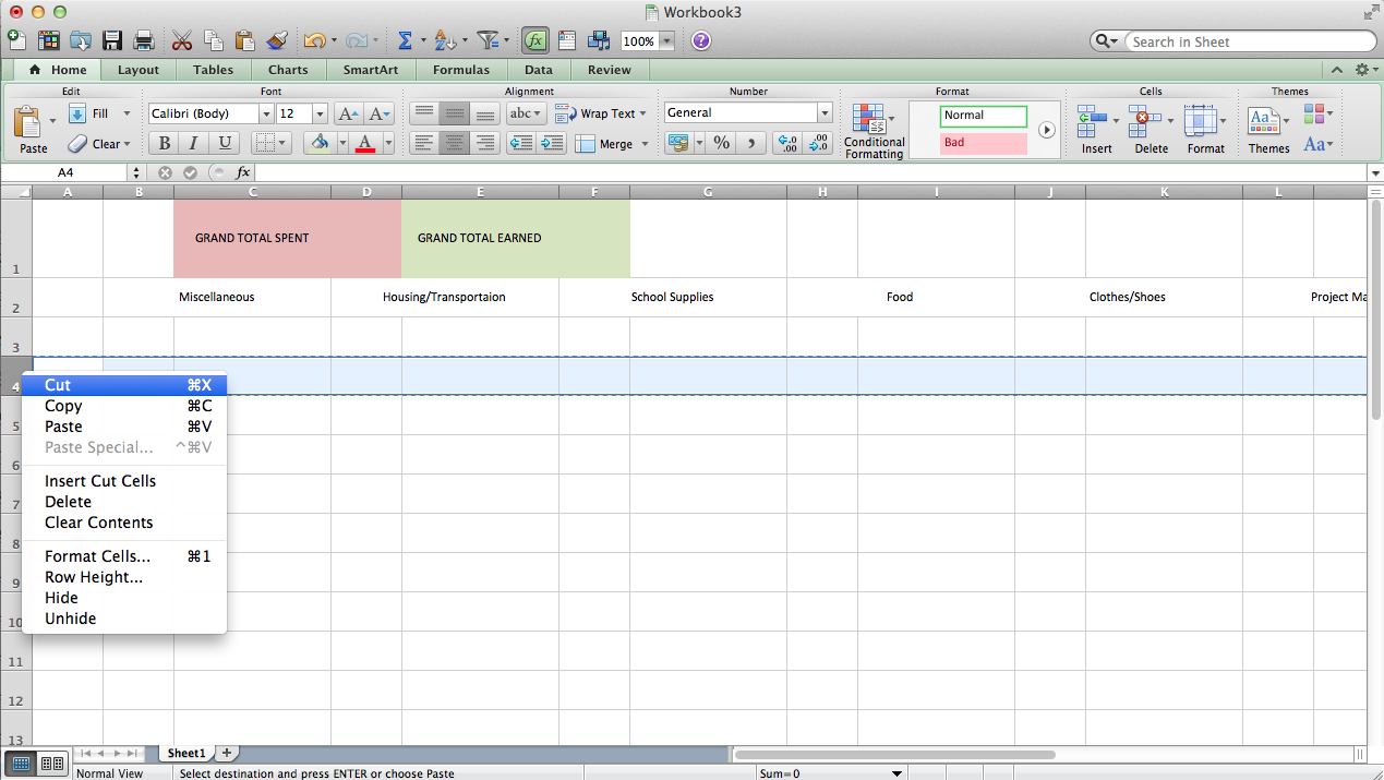
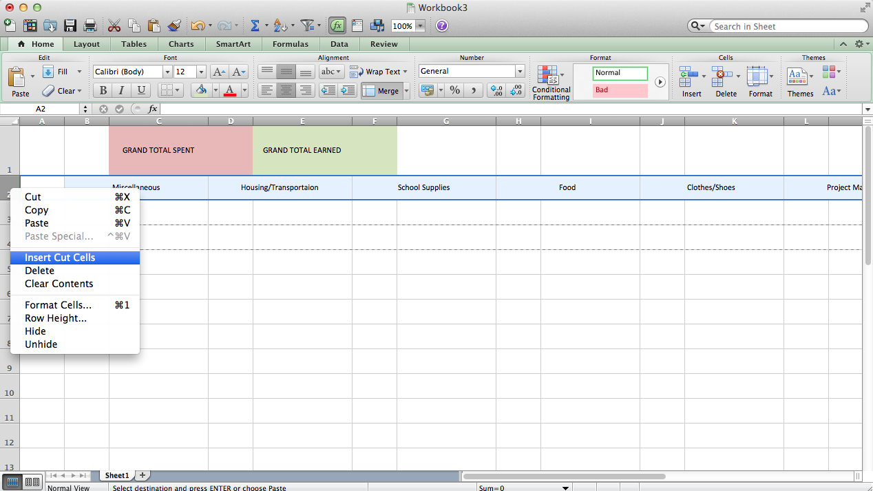
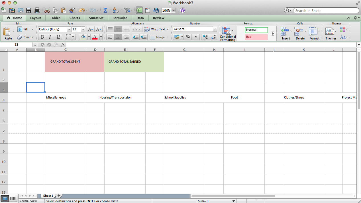
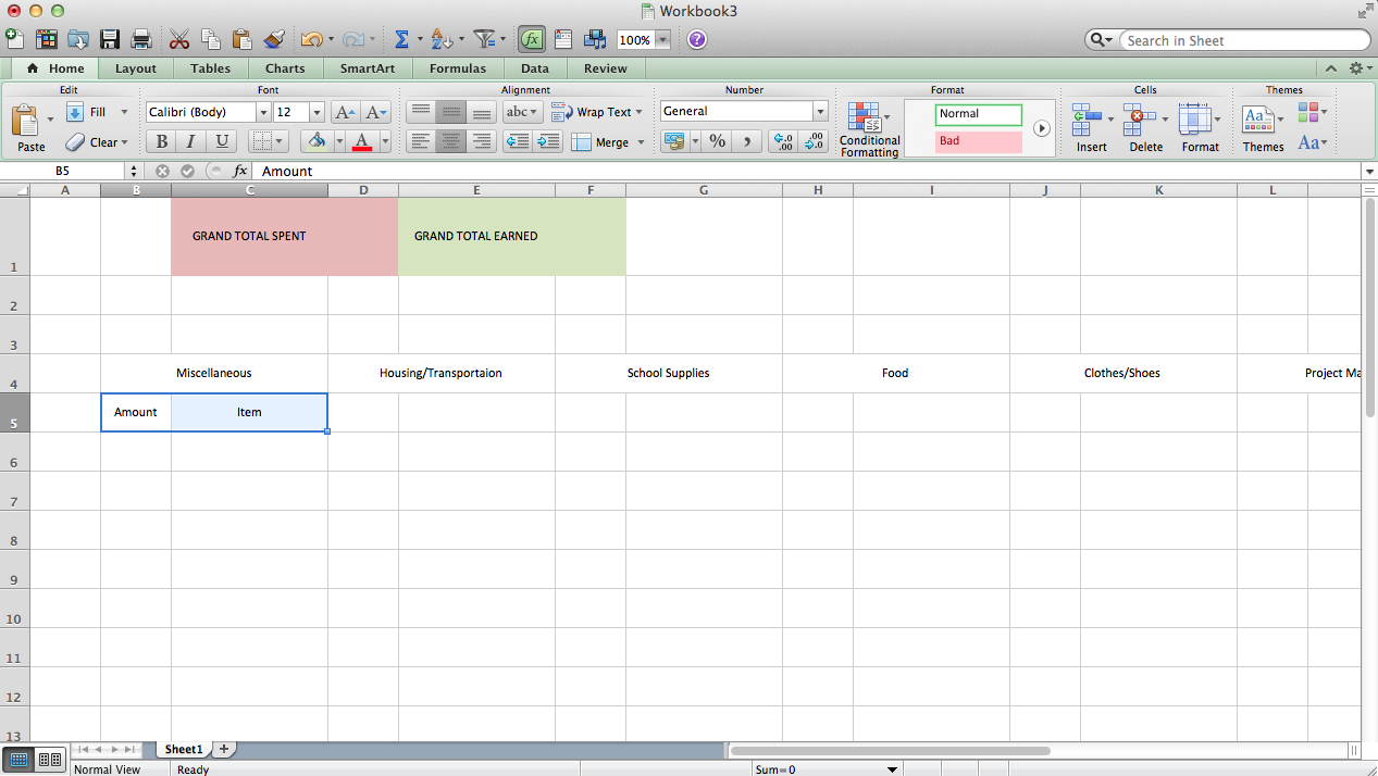
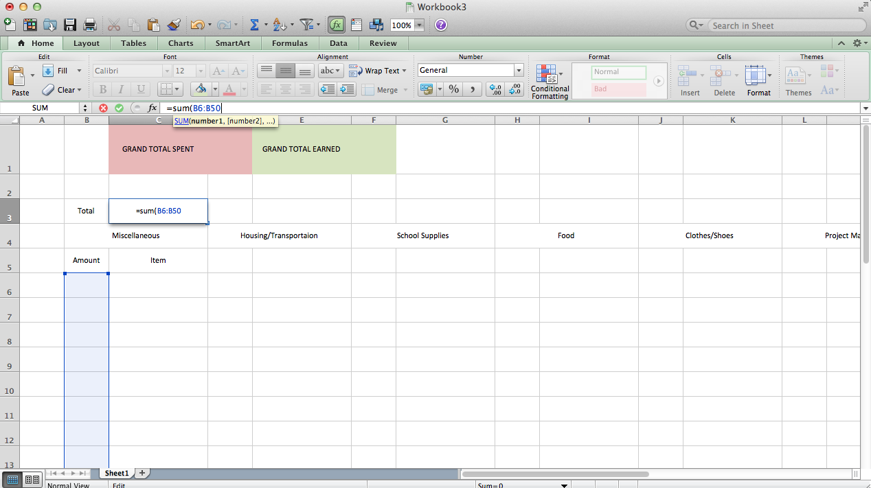
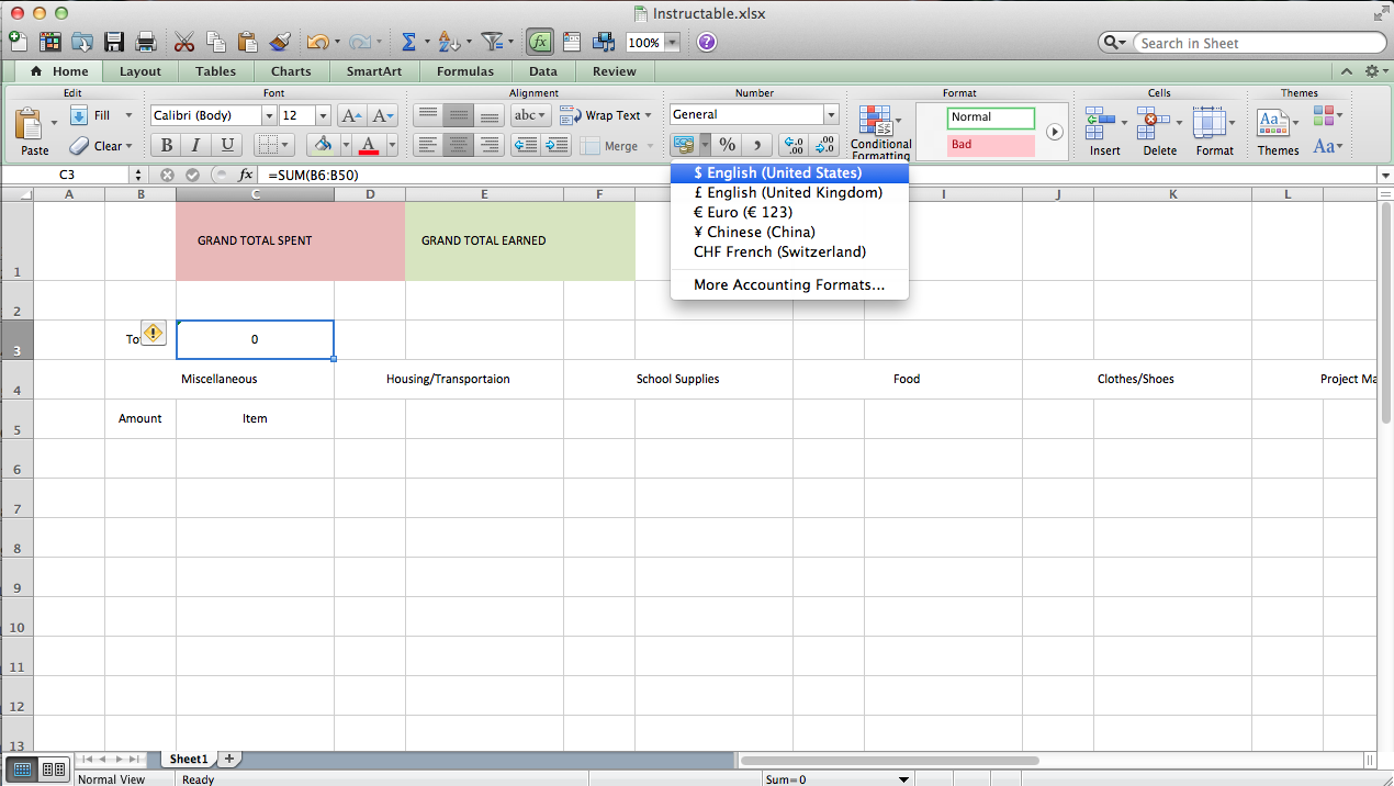
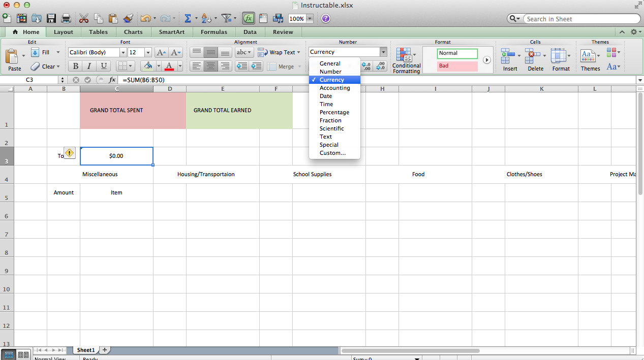
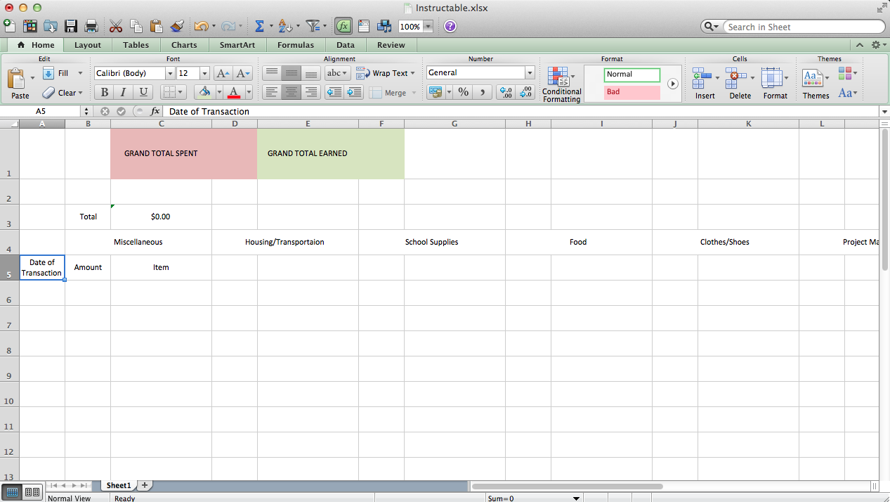
In this step we start typing in some information by labeling specific cells.
Also, see the second picture on centering text! (forgot from previous step)
Quick tip with functions: ALWAYS remember to type in the equals sign before the function (eg. " = sum( "). And if you get stuck in the function (as in when you try to click out, you inadvertently add another cell to the function -- the function bar will say something like " = sum(C4:C70 + L18) " if you selected L18) just press enter to exit out. Then press on the cell with that function and click on the function bar to edit it, before pressing enter to exit again. Otherwise whatever your mouse clicks will be added to the function.
Note: see the pictures above for step-by-step information (easier that simply typing them out here, plus you get a pictorial guide as you go along..)
Highlighting: Part 1
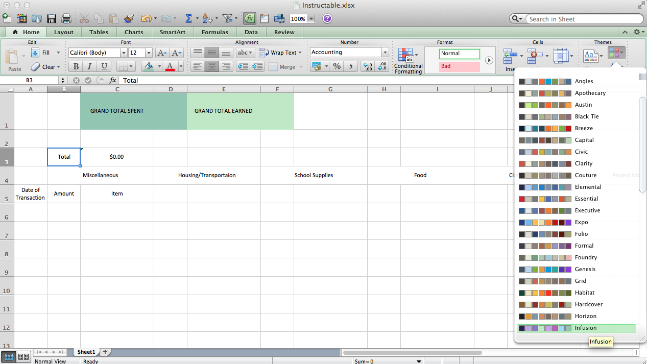
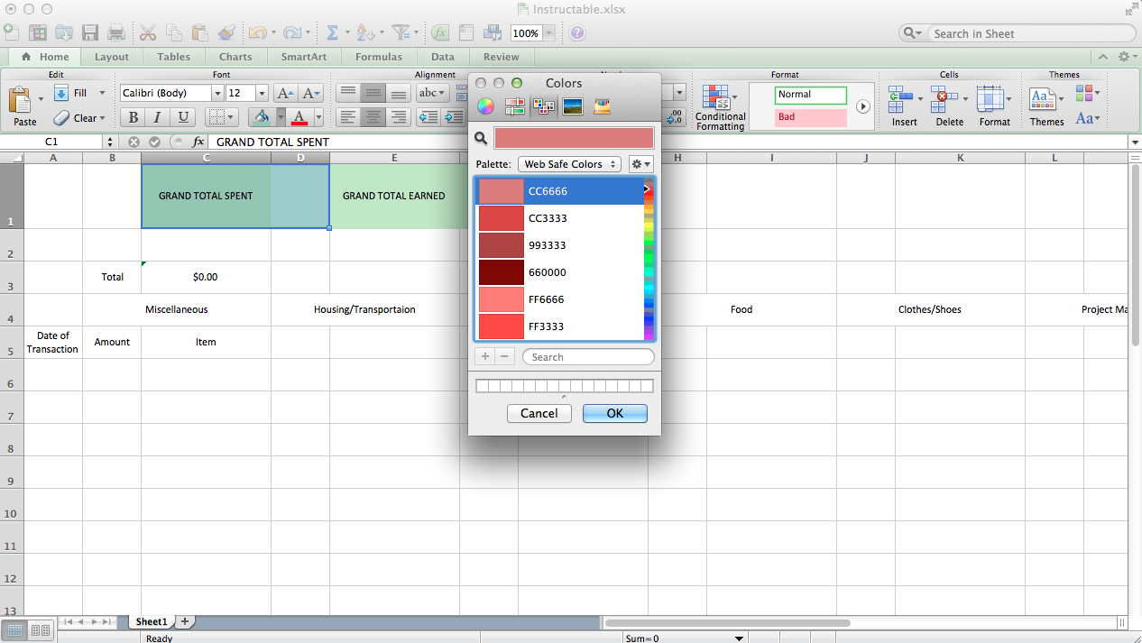
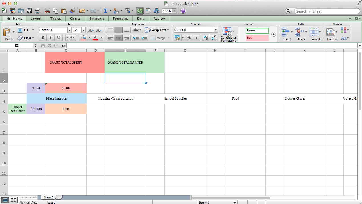
Now we can autofill more cells and add a coloring scheme.
Again, see the pictures above for step-by-step information (easier that simply typing them out here, plus you get a pictorial guide as you go along..)
Highlighting: Part 2
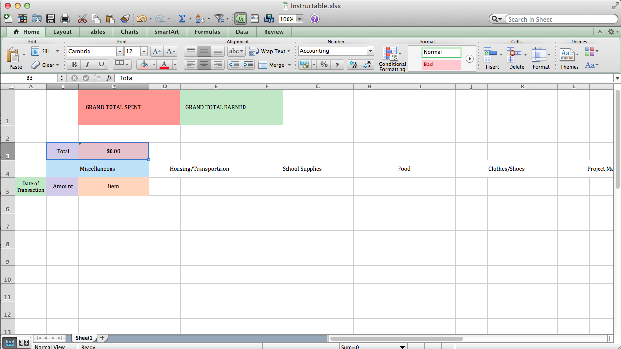
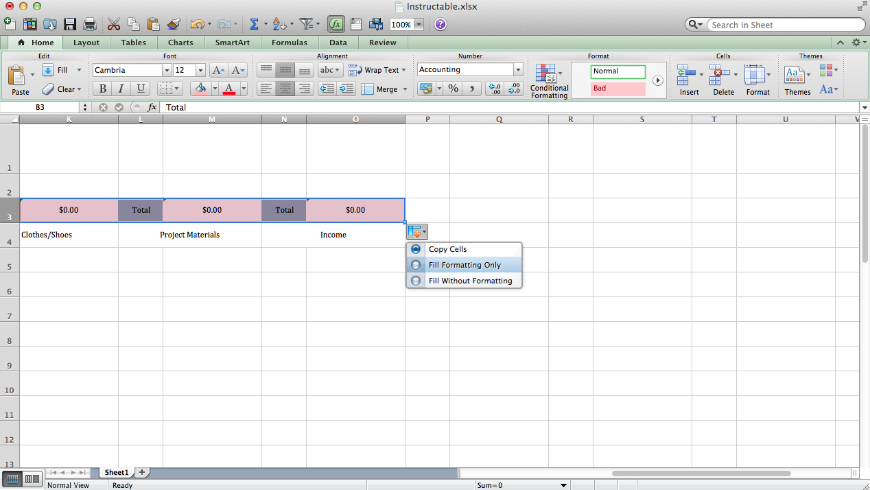
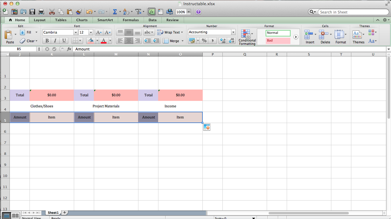
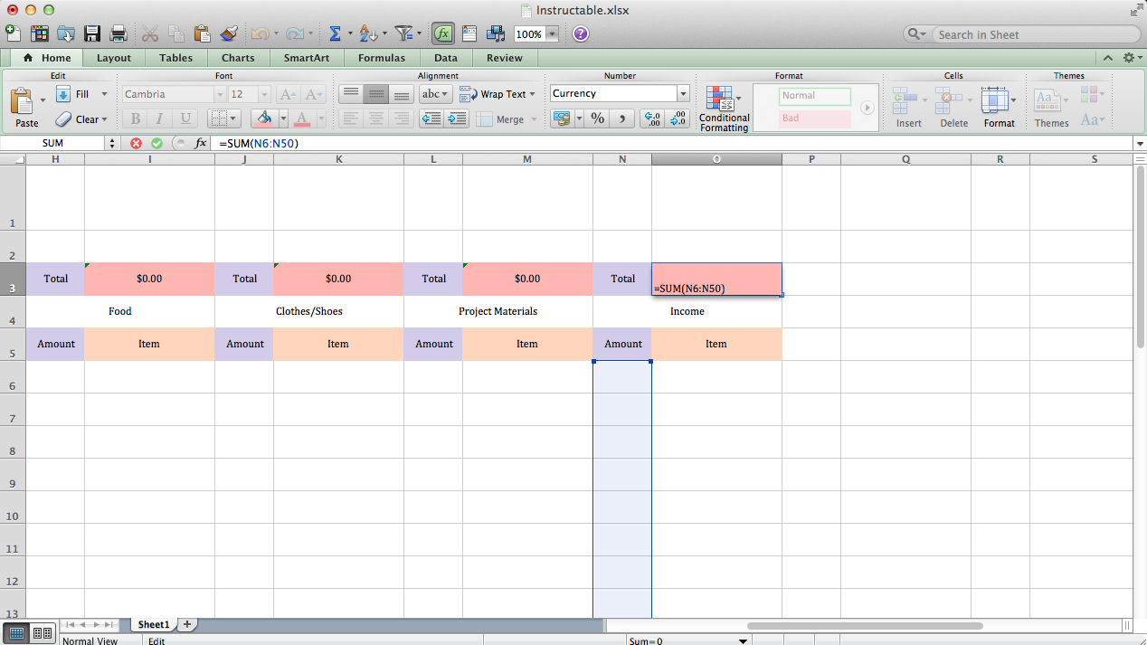
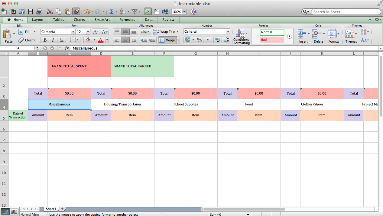
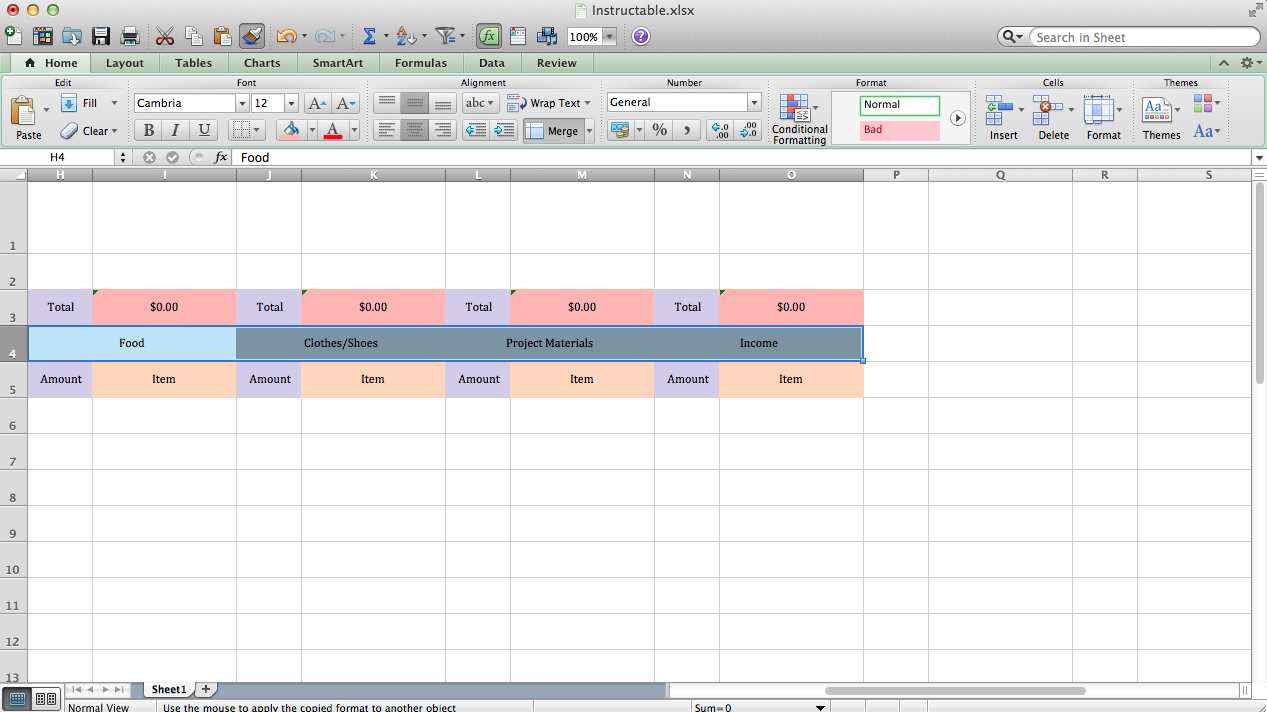
To spread the highlighting to other areas too, we use a combination of autofill and formatting painting.
Again, see the pictures above for step-by-step information.
Text Formatting
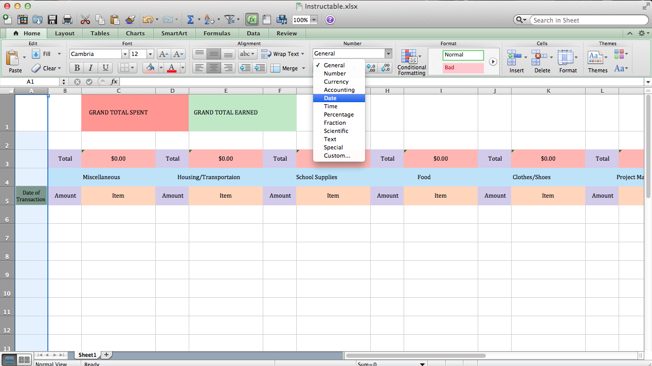
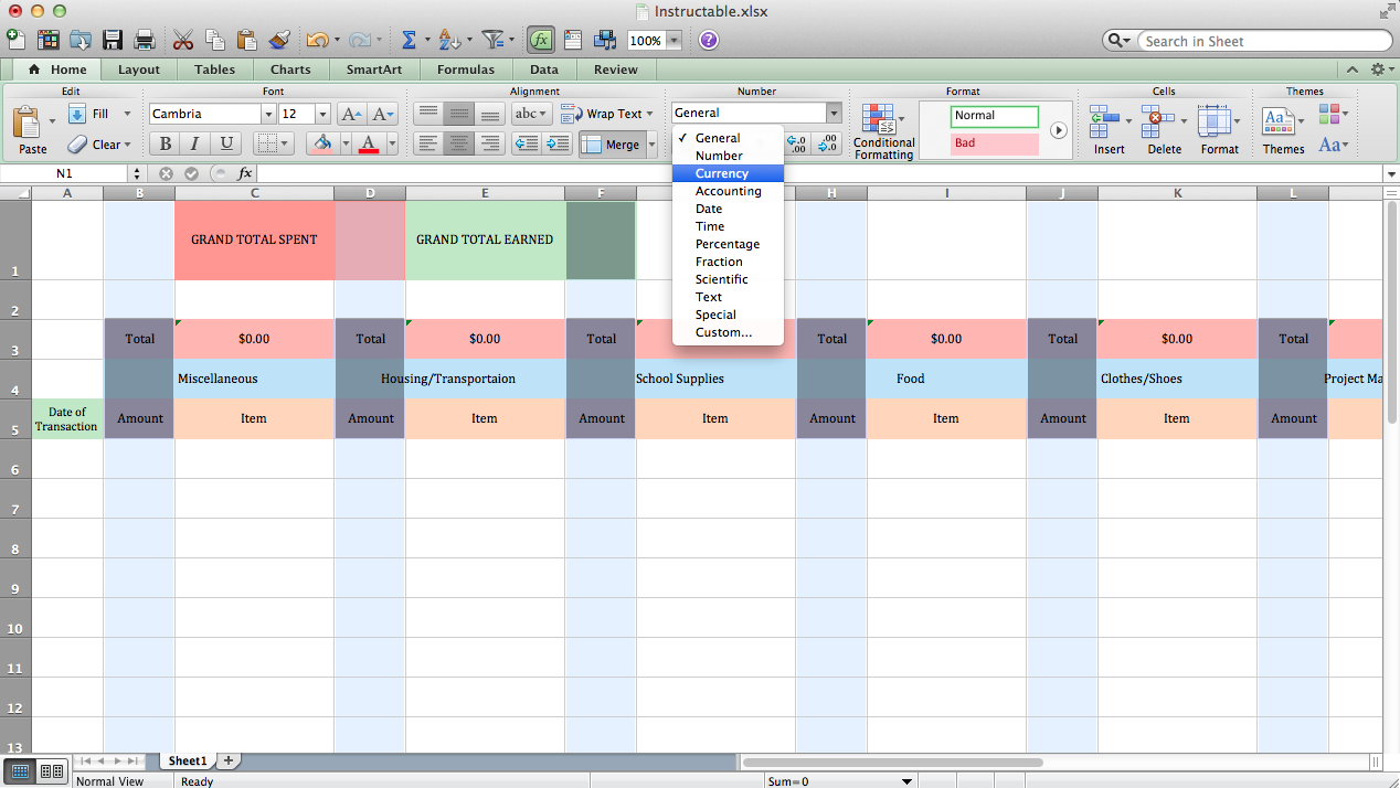
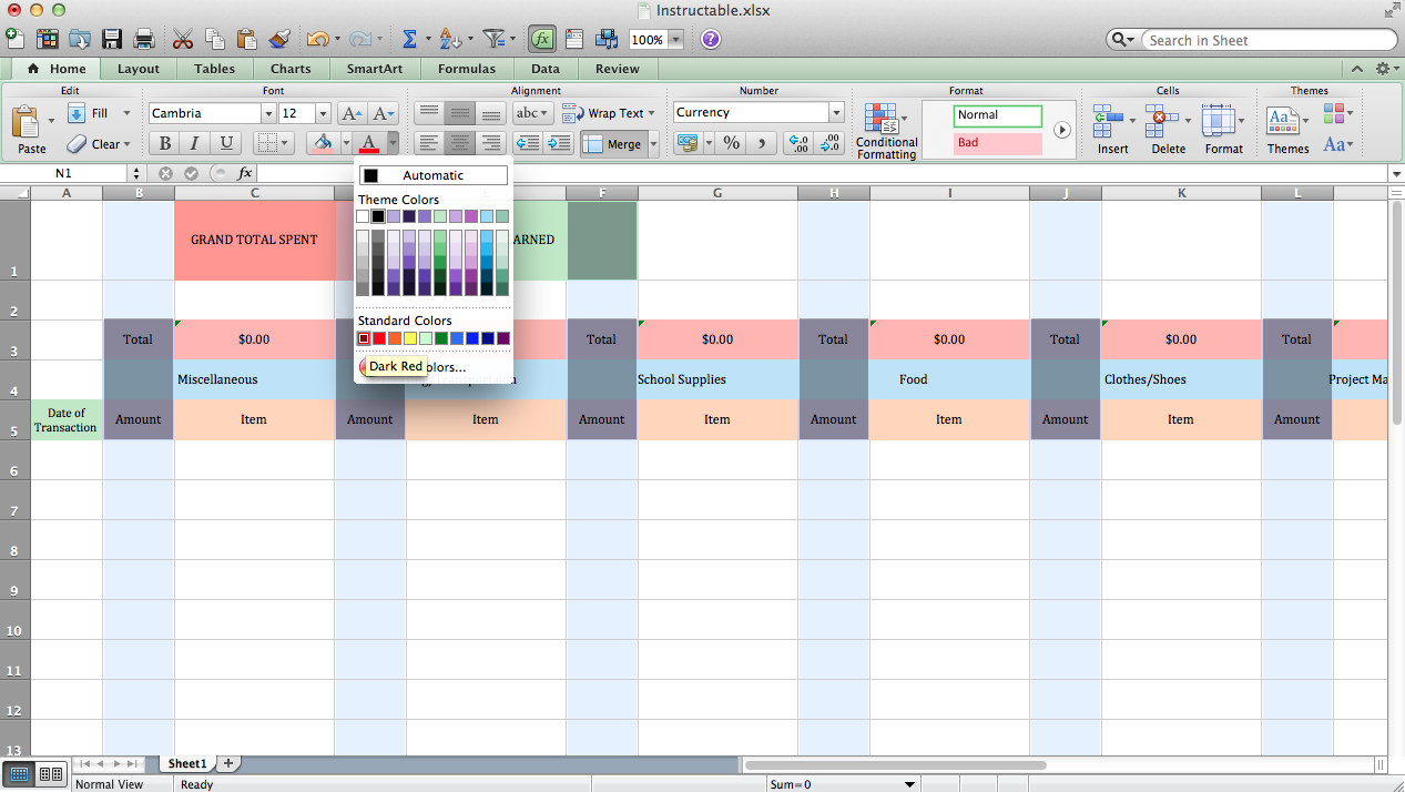
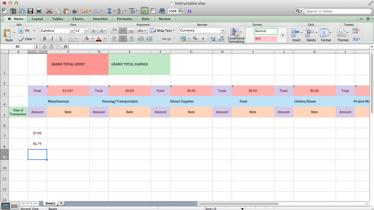
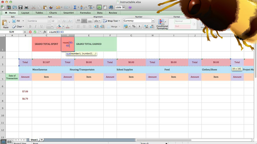
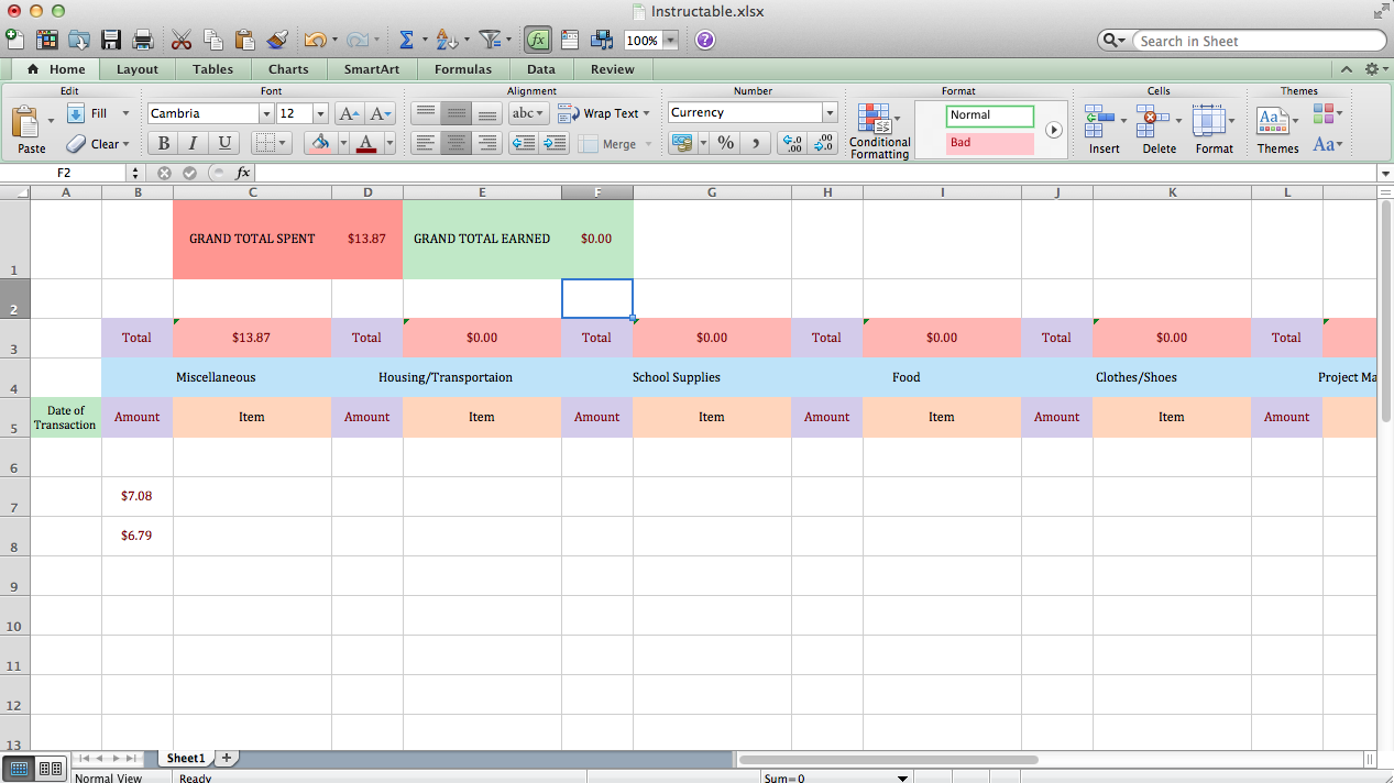
Next step is to change the formatting of the cells, so that the date column's numbers are automatically formatted to a date format, and the amount columns are automatically input in the dollar $0.00 format (and in red).
Again, see the pictures above for step-by-step information.
Grid and Freezing
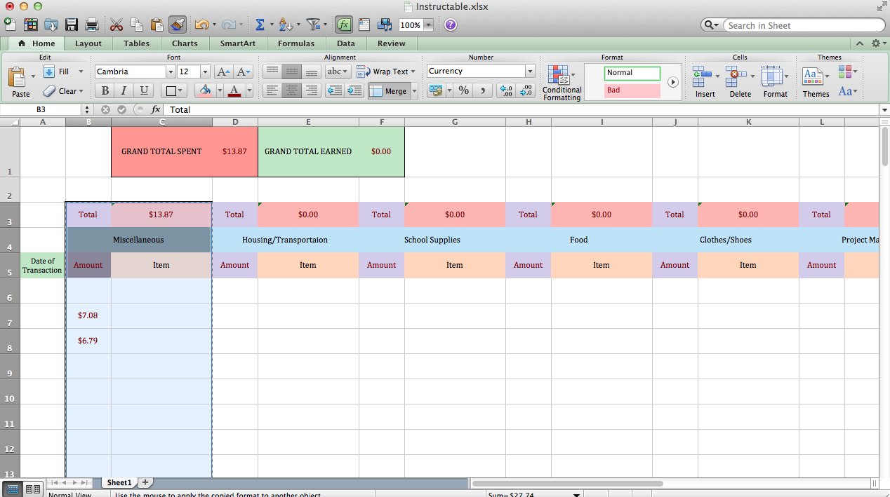
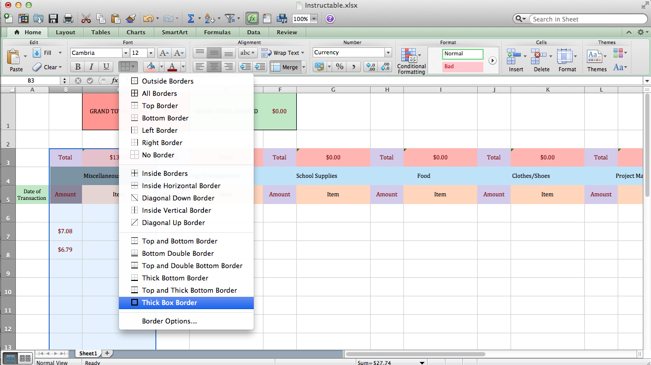
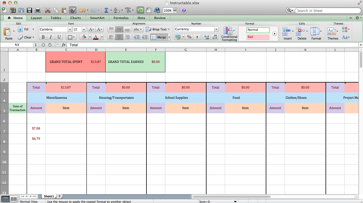
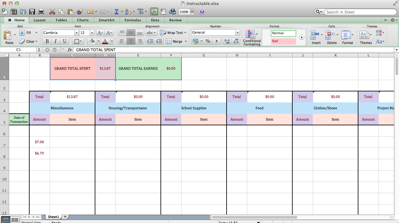
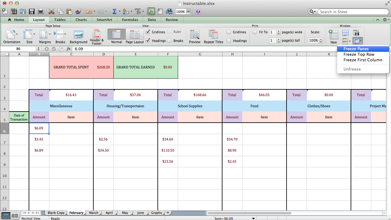
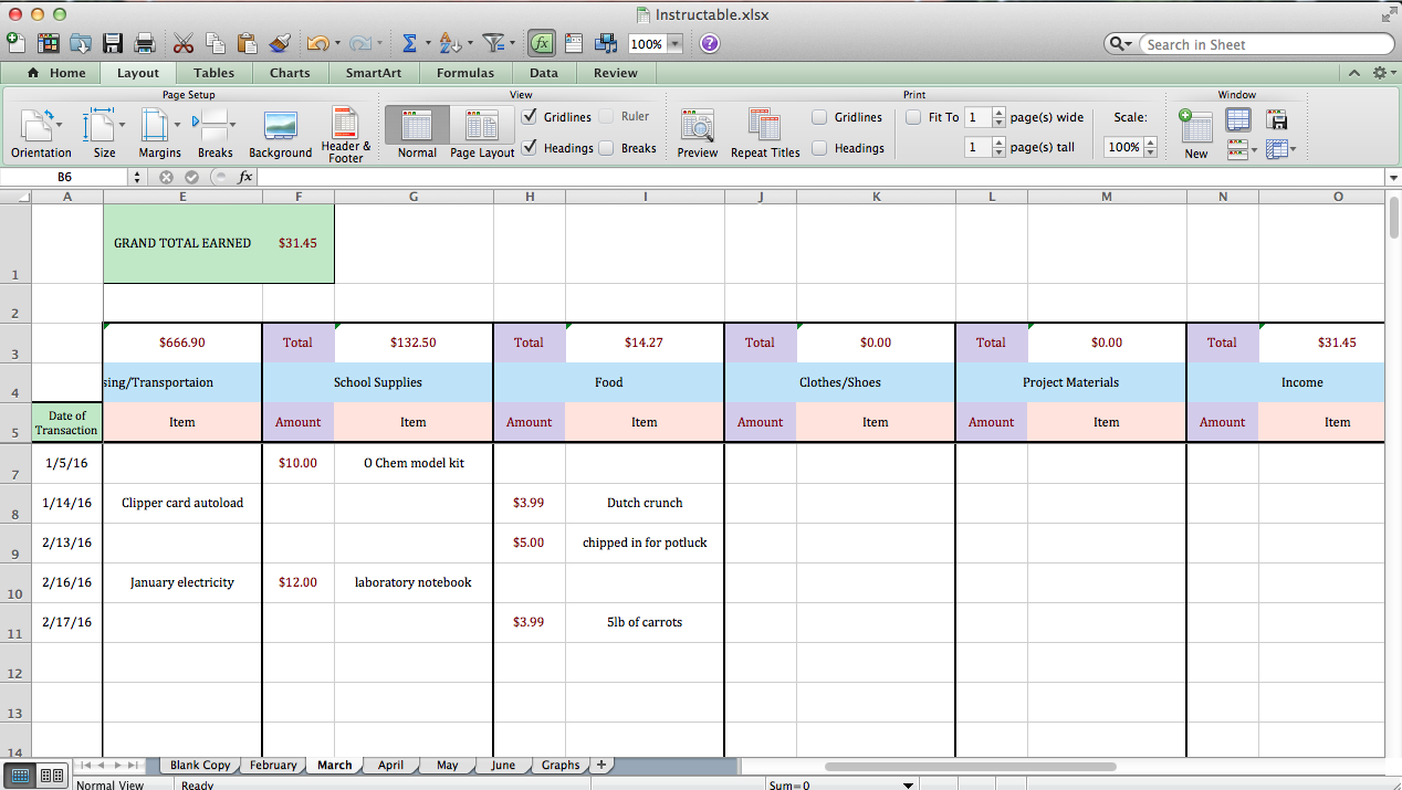
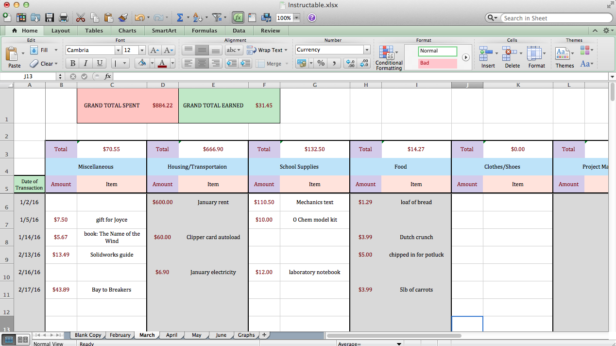
I like to add a nice solid grid to separate groups of cells. Do so by using the grid button as shown above.
Also, you can freeze panes of the spreadsheet that won't move as you scroll up/down/left/right. This allows you to always see the left or top rows/columns.
Again, see the pictures above for step-by-step information.
Conditional Formatting
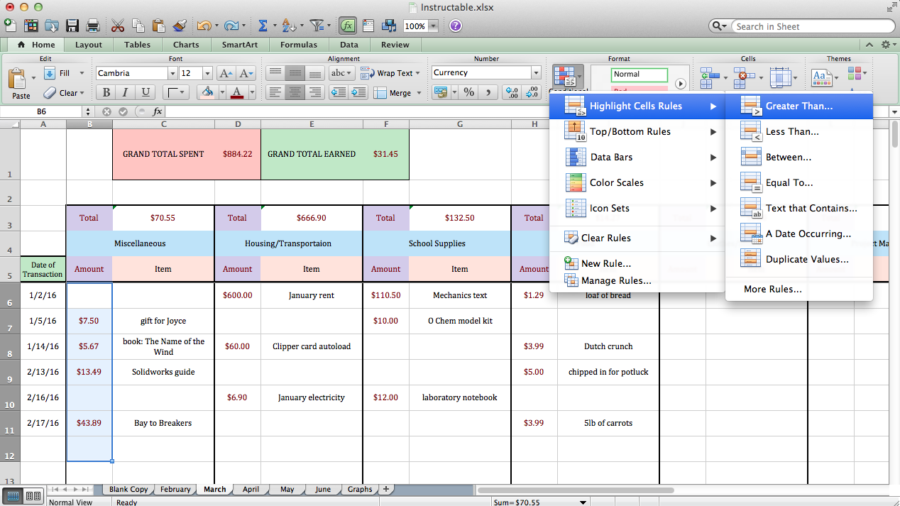
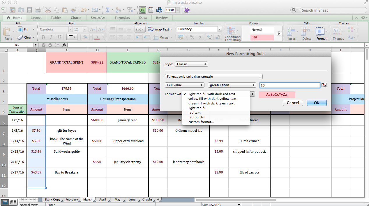
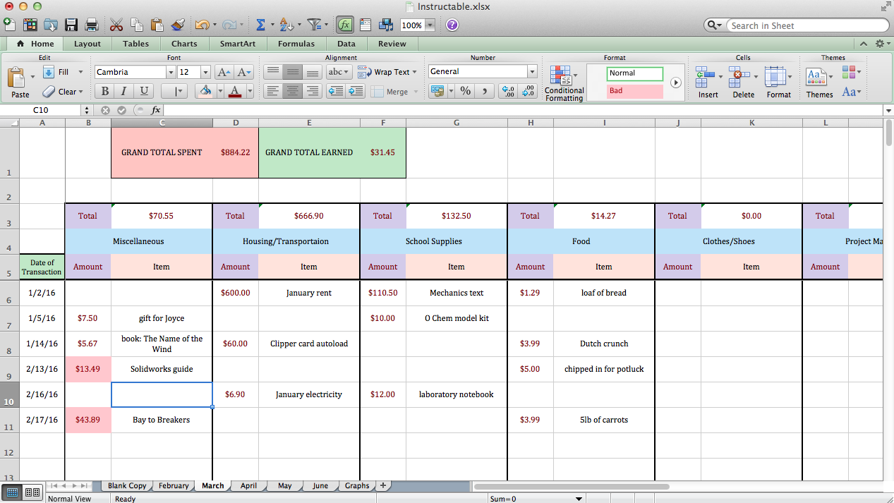
A handy tool with Excel is conditional formatting. You can automatically highlight cells that meet a certain criteria (eg. if you want to be alerted every time you spend over $20 on any transaction, it'll be automatically highlighted.
Again, see the pictures above for step-by-step information.
Multiple Tabs
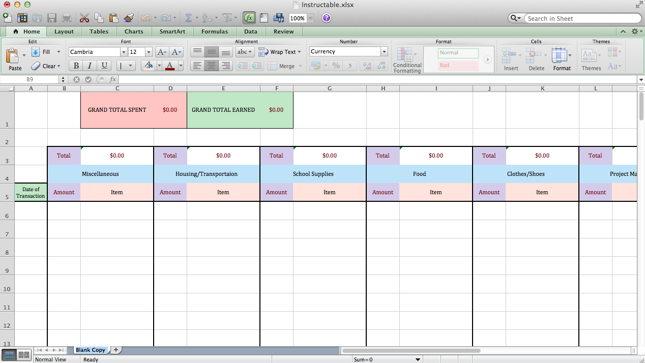
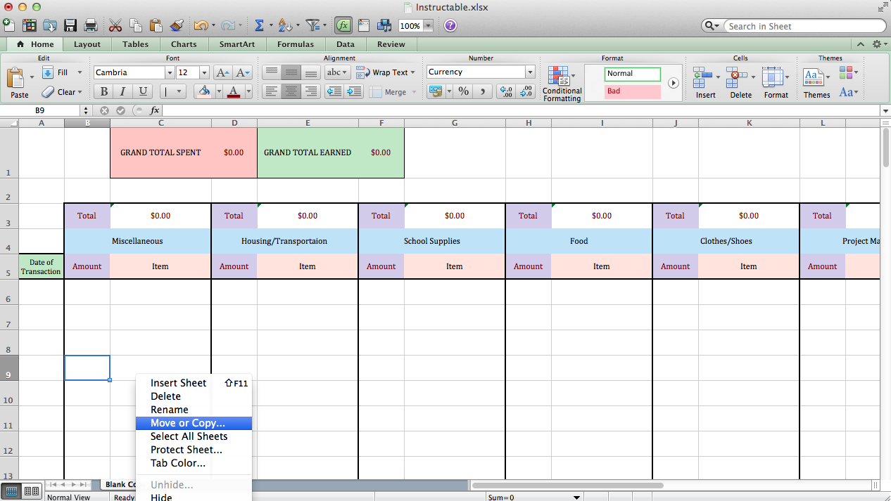
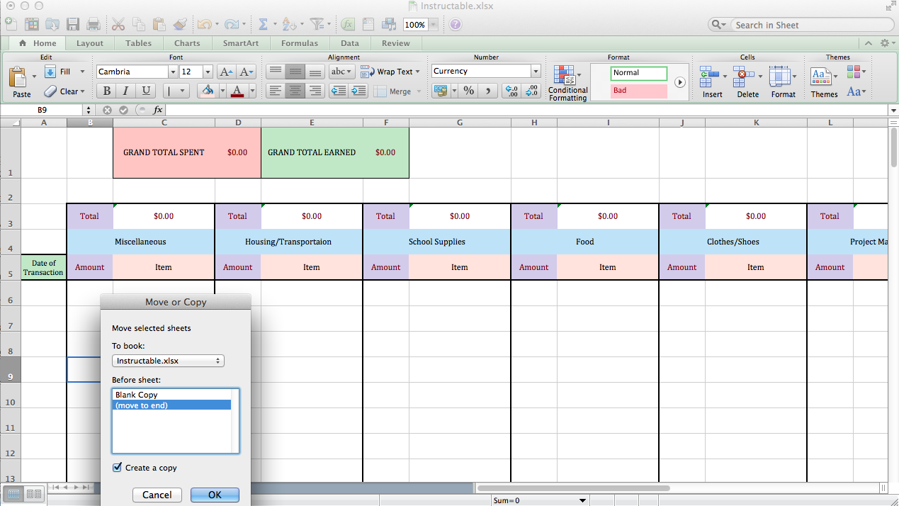
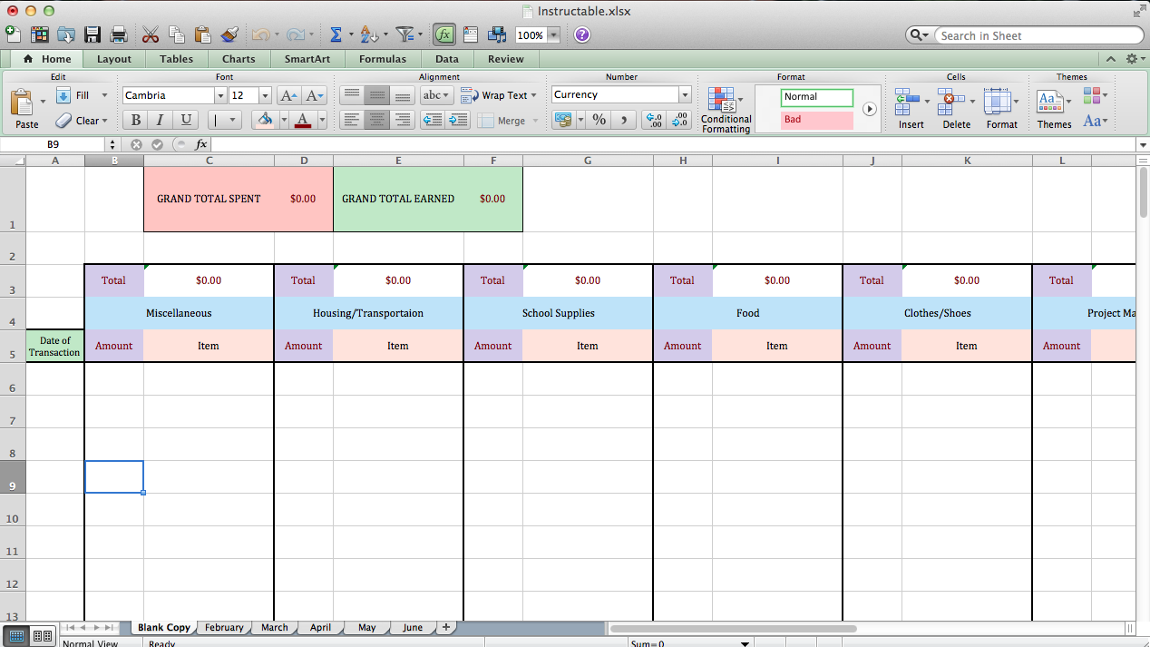
Because I don't want to have a new spreadsheet for each month, I just add another tab in the workbook for each month.
Again, see the pictures above for step-by-step information.
Graphing and Other Additions
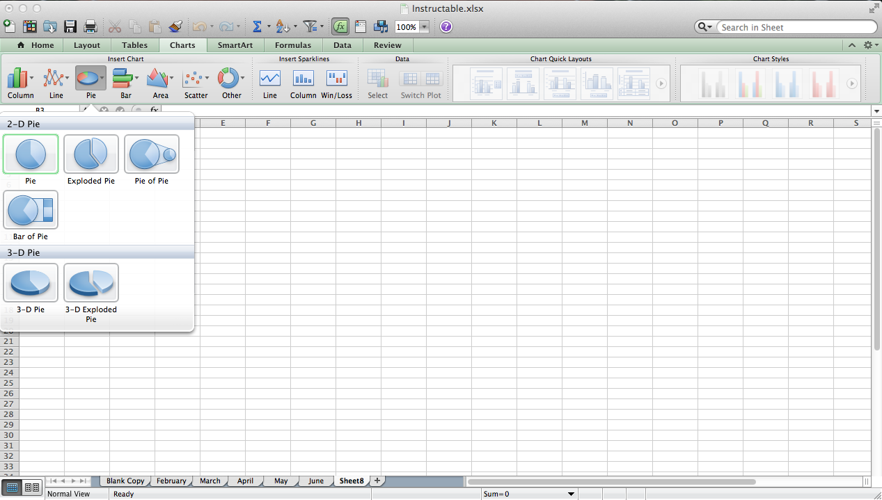
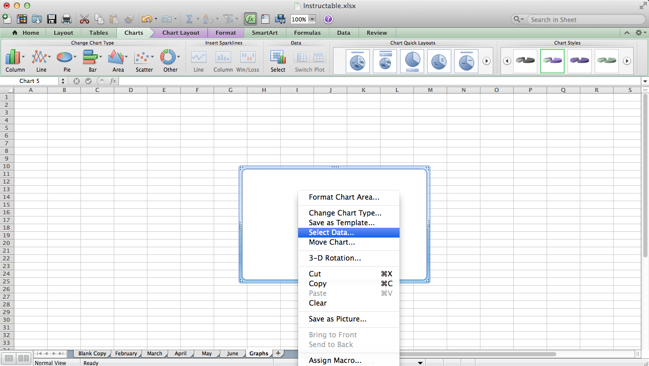
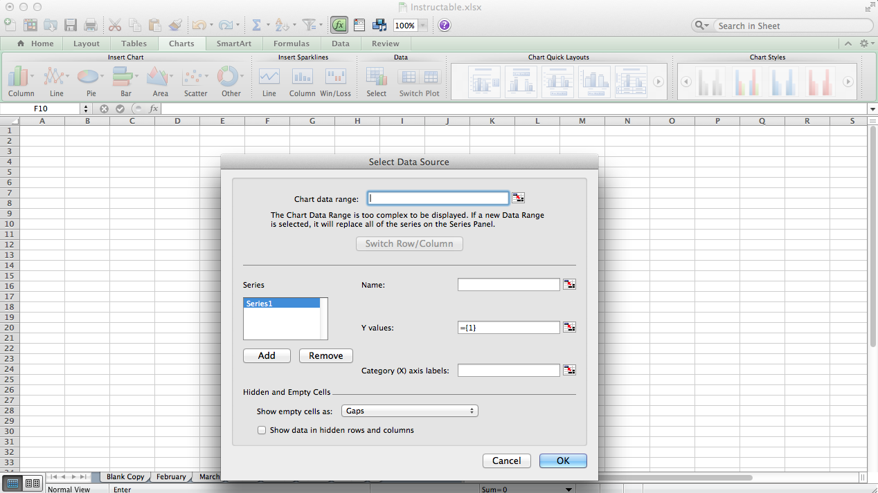
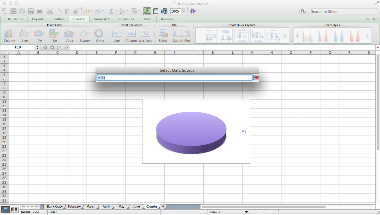
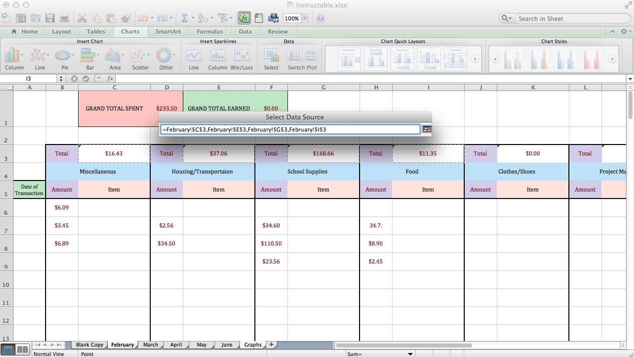

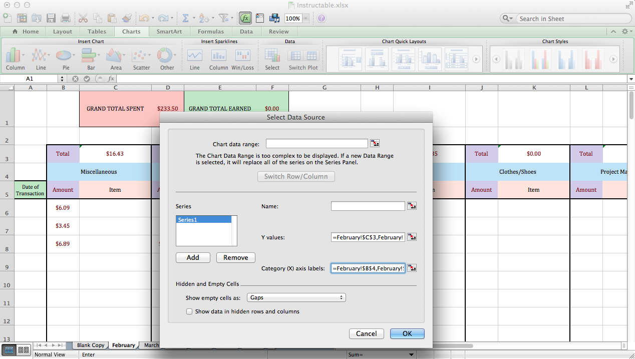
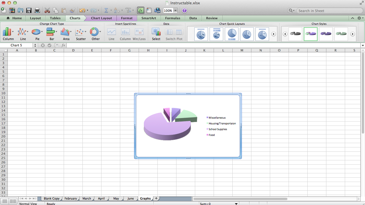
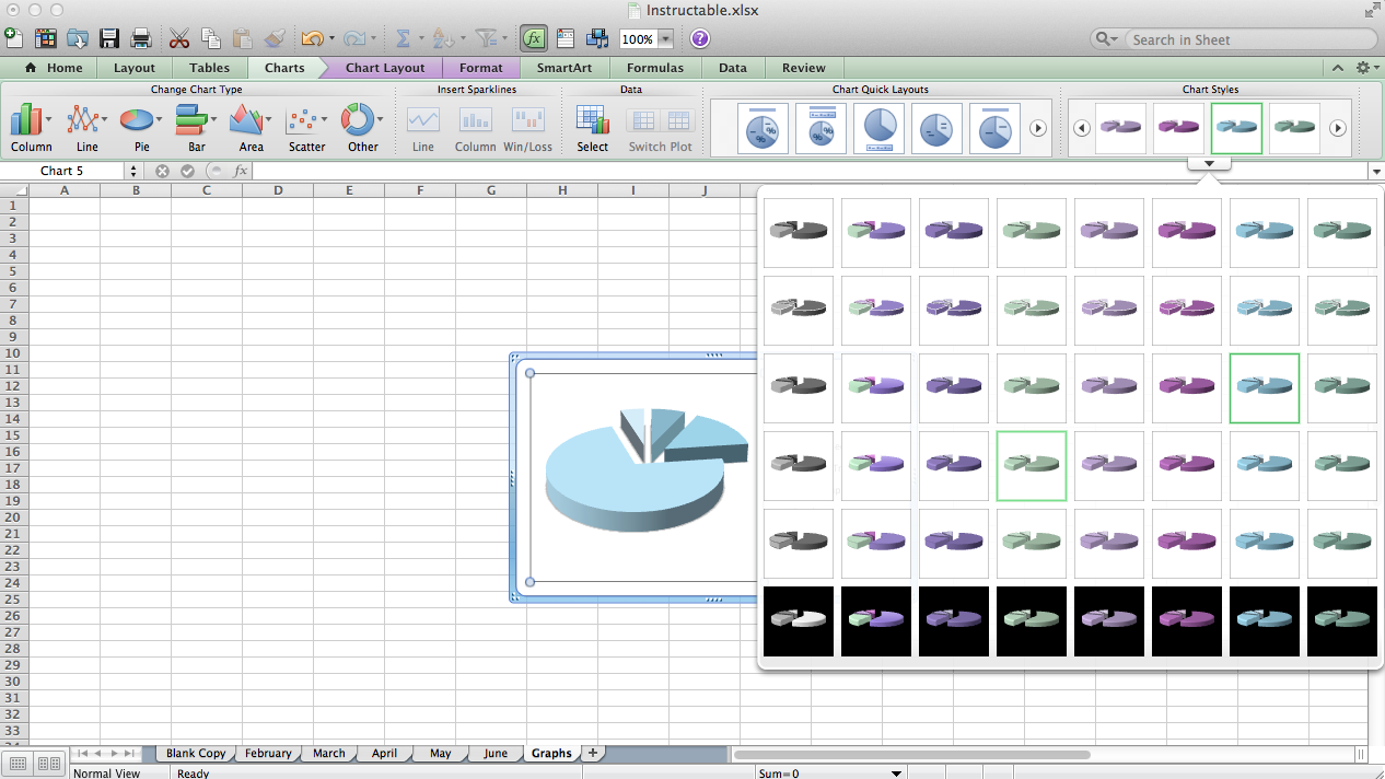
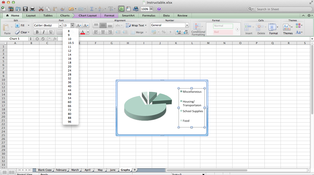
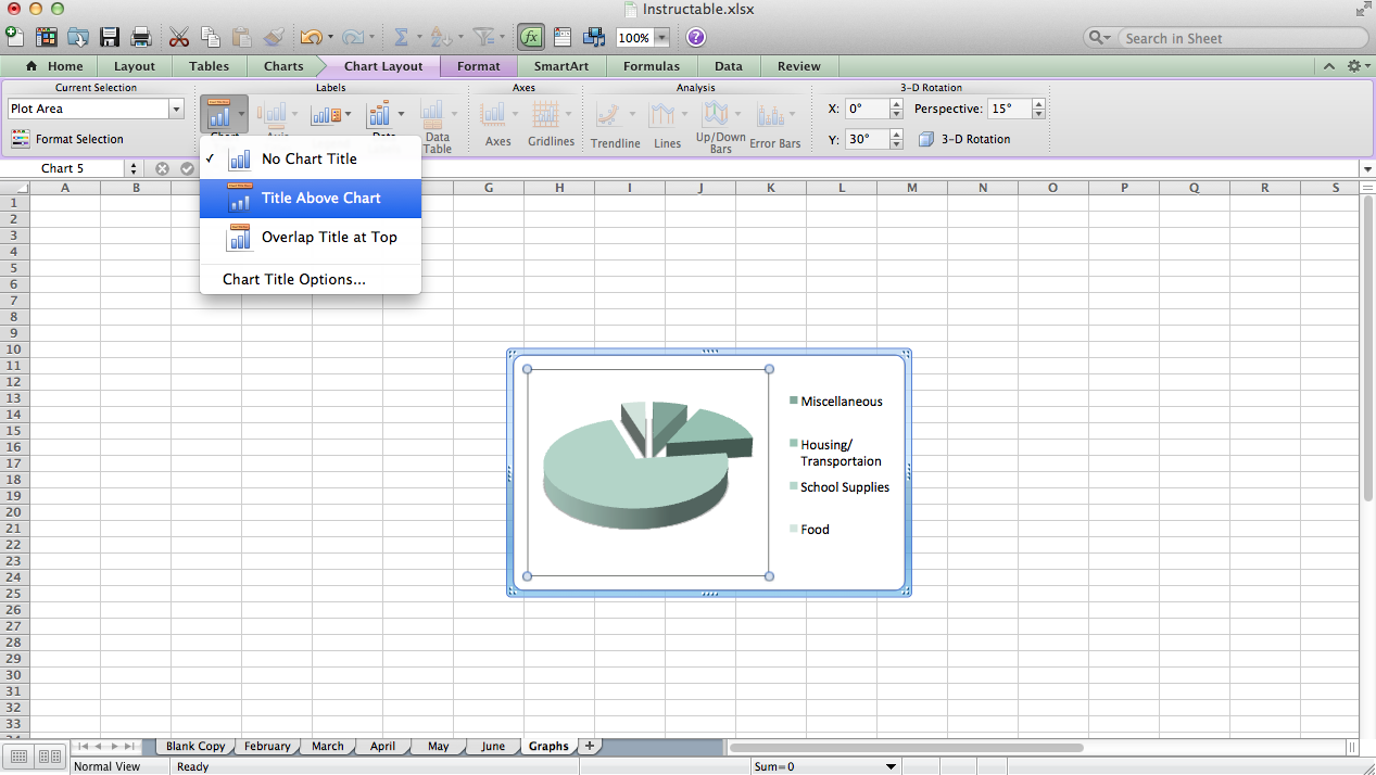
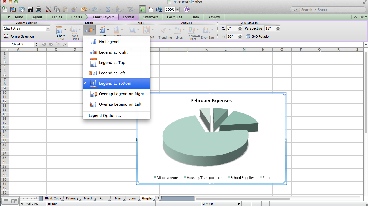
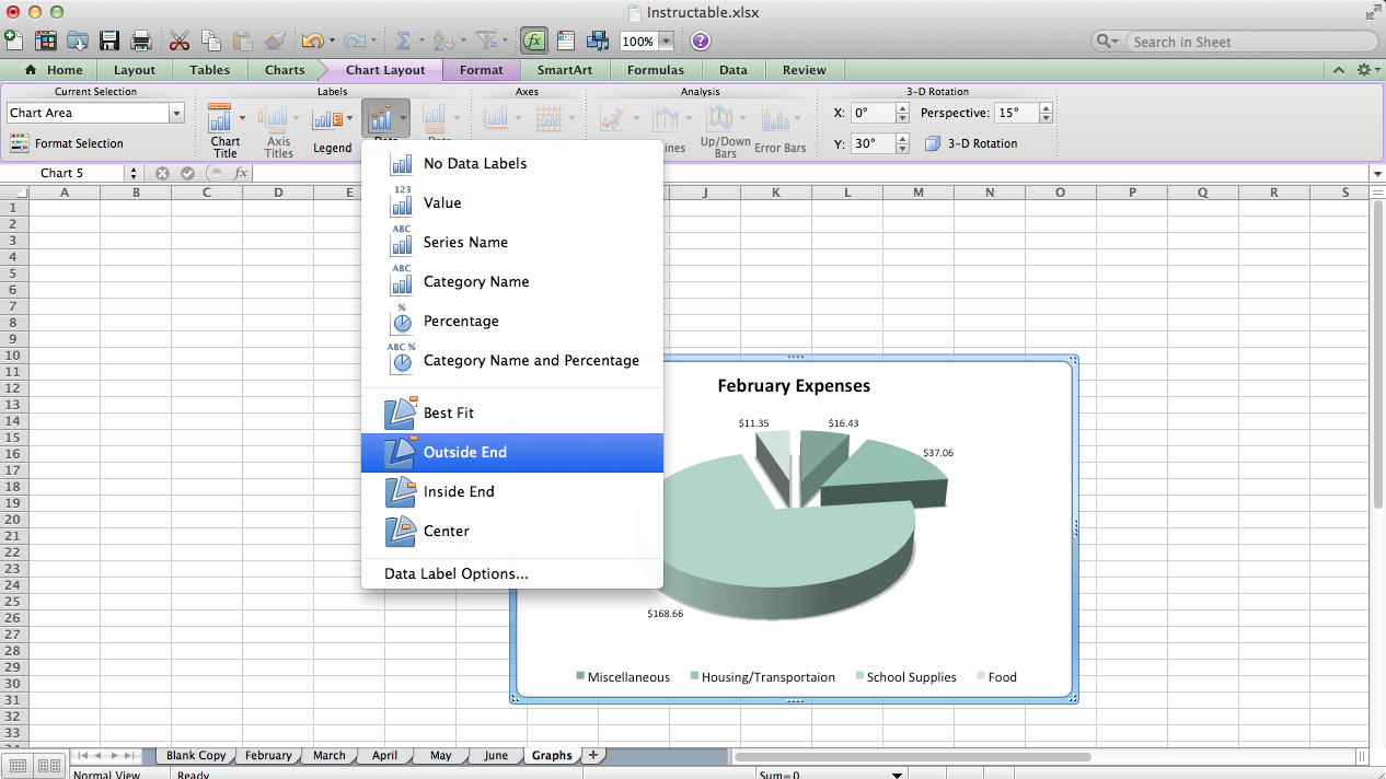
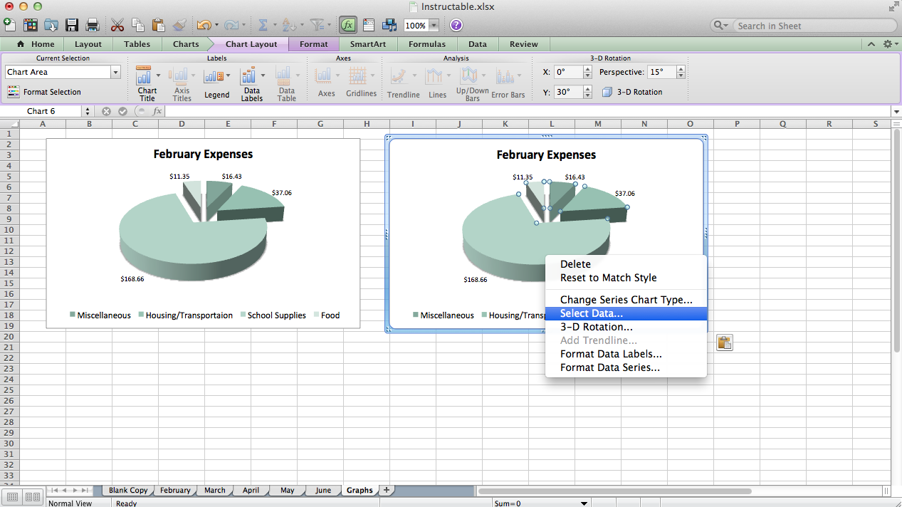
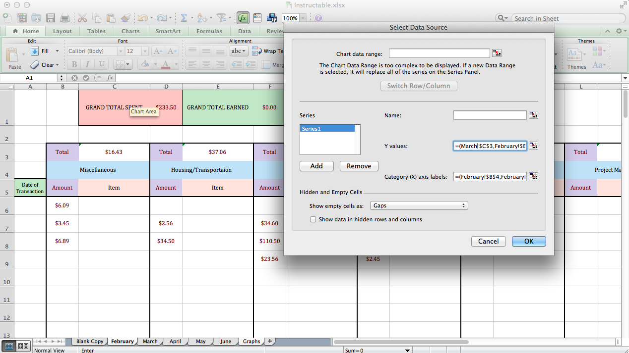
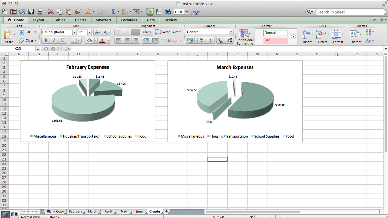
To get a pictorial understanding of your money flow, a graph or two might help. Go to the Charts tab to access graphing programs. Here I've demonstrated the classic pie chart, but line graphs, column tables, etc. are other options to explore.
For charts and data selection, BE VERY CAREFUL NOT TO PRESS ANY OF THE ARROW BUTTONS! THE COORDINATES OF THE CELLS WILL BE ADDED TO THE DATA LINE IF YOU PRESS ANY ARROW. (see pictures for more details)
Again, see the pictures above for step-by-step information.
Filling Out
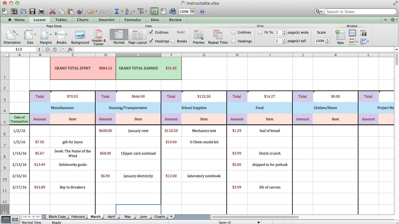
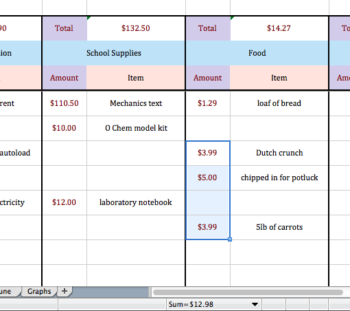
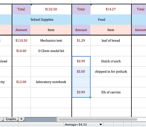

See above pictures on a small overview to fill everything out.
Saving and Finished
You can save this tracking spreadsheet on your computer, flash drive, floppy disk, CD -- anything you so desire, but I highly recommend putting a copy online or in a cloud as backup. Google Drive is a great, free option, and you can even download the Google Drive app on your computer so that it automatically syncs online as you update the sheet in Excel (more details here). Dropbox and OneDrive are great alternatives to that too, as they also have the auto-syncing app feature for computers.
That's your basic expense tracker! Add other features as you like. I know that my formatting doesn't suit everyone's tastes and needs, but hopefully you've learned enough from the previous steps to customize spreadsheets on your own.
Additional Applications/resources
Beyond tracking expenses, Excel is used in many industries to track data of all sorts, for client information to experiment details. For example, I work at a cell culture lab, and we track substance consumption and cell viability for experiments on complex spreadsheets, among other functions. Bottom line: Excel has many capabilities to explore.
I am far from being an expert. Everything I've discussed in this tutorial comes from learning from trial and error mistakes and reading guides during daily commute. You, too, can become more experienced with spreadsheet programs by experimenting more on your own and reading up on Microsoft guides. I found the Office 2013 for Dummies book particularly helpful, and most libraries have at least some version of it for other years. You can pick up an older addition for fairly cheap (new version are great, but you can save ~70% of the cost by getting the previous editions -- college textbook tips...) if you like to highlight and bookmark.
I hope this tutorial comes in handy for others, and have fun! If anything is unclear, feel free to comment below, and I'll help to you if/when I can.