How to Model a Simple Spring-Mass-Damper Dynamic System in Matlab

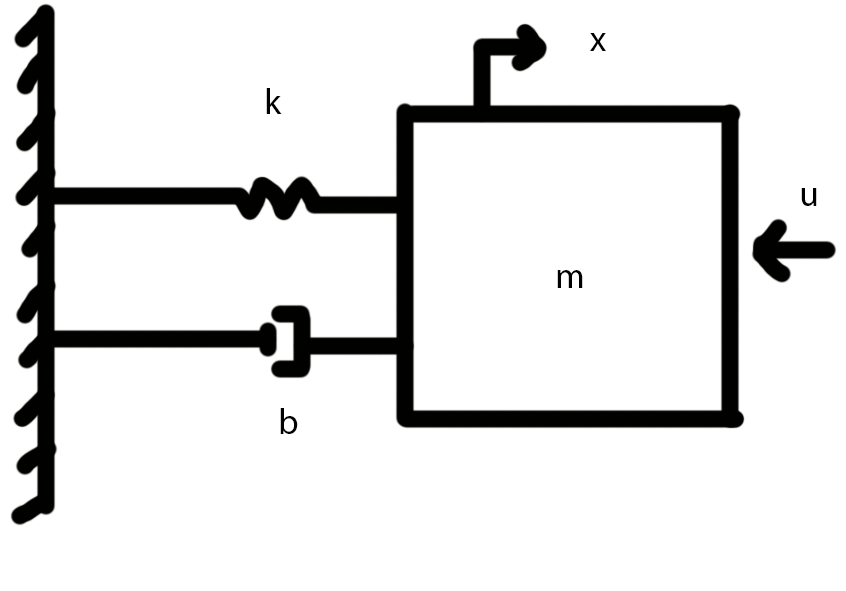
In the field of Mechanical Engineering, it is routine to model a physical dynamic system as a set of differential equations that will later be simulated using a computer. These systems may range from the suspension in a car to the most complex robotics. The aim of this Instructable is to explain the process of taking a state-space system and simulate the step response using Matlab. To do this, the mass-spring-damper system shown above will be used as an example. There is no training required to complete these steps, however to fully understand the procedure a background in mathematics is advised.

In order to understand the steps to follow, one must first understand some of the terminology that will be used. First, a dynamic system is anything that changes with time. This could be a pot that heats up on a stove or a speaker that plays music when an audio signal is applied. The second thing to understand is that dynamic systems can be modeled using a branch of mathematics known as ordinary differential equations (ODE's). Knowing how to solve ODE's is not important to complete this series of steps, but it should be understood that they are a mathematical model. ODE's can be written in a variety of forms, however to simulate systems in computer software it is convenient to use something called the state-space form. State-space form is a way to organize ODE's such that there exist 4 matrices containing the relevant system properties. Lastly, by using a computer program called Matlab, one can simulate the system with respect to a variety of inputs. Matlab is a linear language that executes each command line at a time. The steps mentioned in this Instructable are set up in such a way that each new line of code will be entered into the next available line.

Verify that Matlab is installed on the computer in use. If the software cannot be found, try searching for it using the bar at the bottom left of the screen. This searching method only applies to the Windows 10 operating system. Once Matlab is open, a new script should be created. This is done by clicking the "New Script" button located in the top left corner of the program. The cursor should be in the editor window and the coding process may begin. Matlab has a convenient feature of telling the user what mistakes have been made. This will happen in two ways. The first is a red line under an error. To learn the nature of the error, hover the mouse over the line. The second will be discovered upon operation. When the program runs, if it encounters an error it will type in red what the error is and the echo the line that the error occurs on.

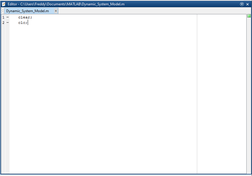
For easy debugging and viewing, type in the following lines of code.

clear;

clc;

This will clear all workspace variables and the output screen before each script execution. While not necessary, this small amount of code will allow a user to easily see any issues with the program and clean up the output. It is important to note that Matlab code is case sensitive.

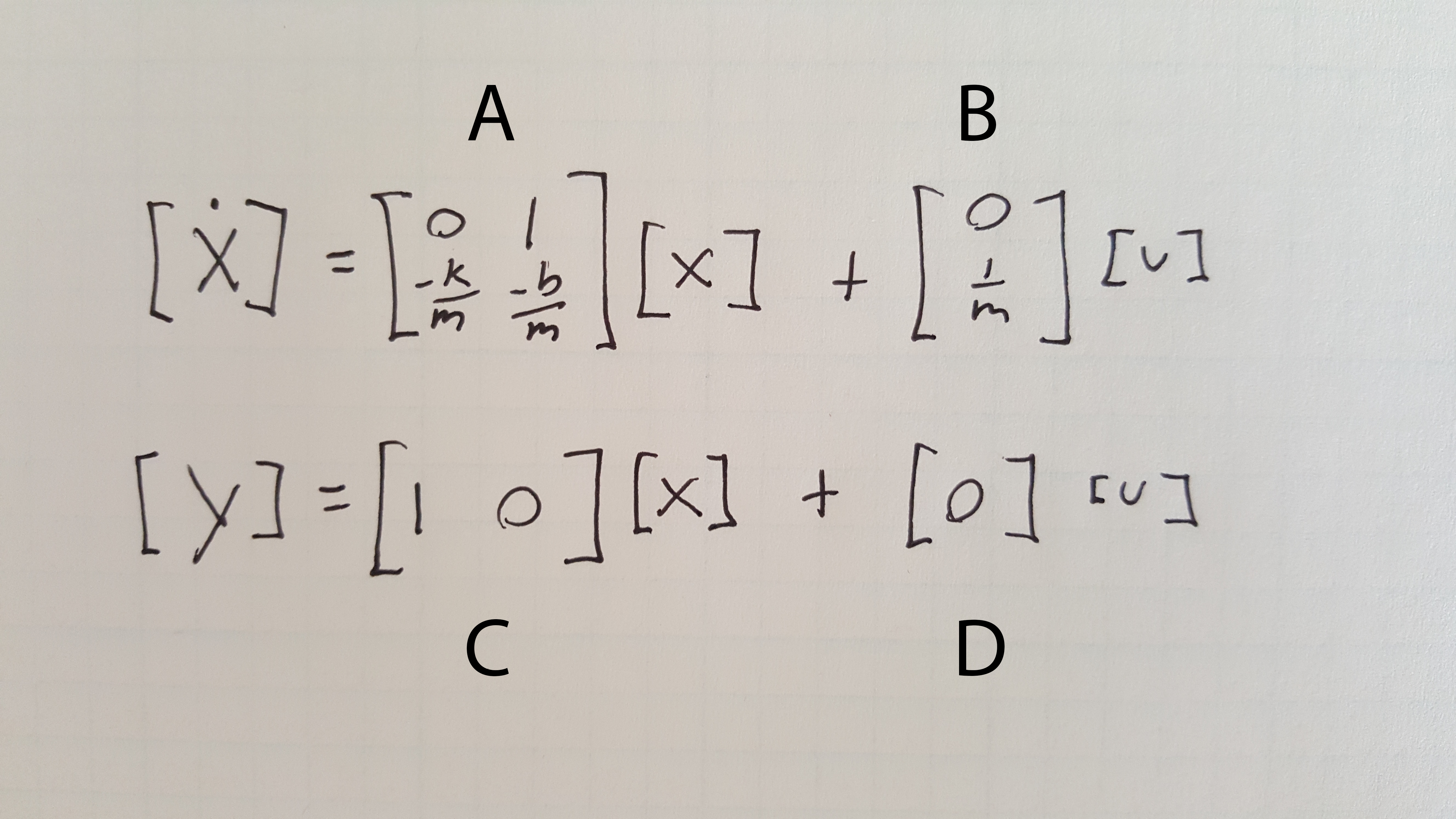
There will always be 4 separate matrices when modeling a system in state-space form. These will be noted as the A, B, C, or D matrix depending on the location in the equation. Before the state-space matrices will be defined in Matlab, it is good practice to confirm that all matrices are present in the information given. The state-space representation for the mass-spring-damper system is shown here.

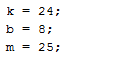
In mass-spring-damper problems there are several numerical constants to note. The constant k is called the spring constant and refers to the rigidity of the spring. The constant b is known as a damping coefficient and is significant in that it helps model fluid resistance. M in this case simply represents the mass of the block. For this simulation we will assume k = 24, b = 8, m = 25. Typically these values would have units associated, but for simplicity they have been omitted. To define these in Matlab begin with the variable name, such as "k," and set it equal to the number associated with it. For example, "k = 24;" is a proper declaration.

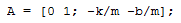
Now that it has been confirmed that the given form is correct and the system constants have been defined, it is time to begin defining the system in the code. To begin, declare a variable called "A". This is done by typing "A = " on a single line followed by the matrix. To code the matrix, open with a bracket and type each term in order from left to right, top to bottom. Each column should be separated by a space and each row by a semicolon. Once the information is entered, close the line with a closing bracket followed by another semicolon. The final result should look something like the picture above.

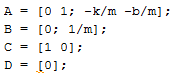
Once the A matrix is coded into the software it is time to define the other 3. The method for this is the same for step 6 with the only difference being that the name, numbers, and size of the matrices may be different. It is important to remember that new columns are separated by a space, and new rows are separated by a semicolon. The final result should look something like the code pictured above.

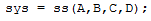
One reason that Matlab is so widely used for dynamic system simulation is that it has most of the hard code already programmed. Now that the state-space matrices have been defined, the entire system can be condensed into a single variable in one line of code. To create a system variable, define the variable like any other using the variable name and an equals sign. In this case, the name "sys" will be used to represent the system. Next, on the right hand of the equal sign type "ss(A,B,C,D);" which will reference a Matlab state-space function. By doing this, the program now recognizes "sys" as a system of ODE's that can be used to simulate a response. When entered into Matlab, this line of code should look like the picture above.

Now that the system has been modeled entirely in Matlab, it is time to see how the system responds to a certain input. In this case, a step input will be used. A step input is an instantaneous change to some constant value, and in this system would signify a force being added to a system at rest. Simply type in the line "step(sys)" to code this in Matlab.

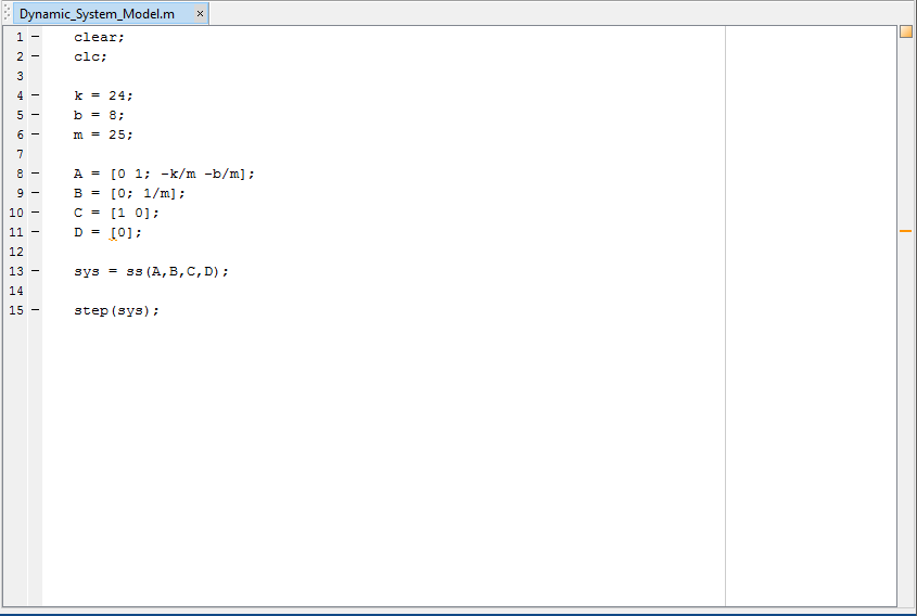
It is important to check that the code entered is correct corresponding to the state-space equations given. Unlike many problems in engineering, even if the wrong lines of code have been entered the code may execute and display information. This is an issue due to the fact that not all information output will be correct. This step exists to force the programmer to walk through the steps a second time with the intent of comparing the code with the instructions looking for inconsistencies. To further check for errors a copy of the final code may be seen above.

Once all steps have been completed and the quality of the code has been verified, the code may be executed. This is done by either pressing the F5 key on the keyboard while the cursor is inside the editor block or clicking the "Run Section" button located at the top right of the Editor Tab.

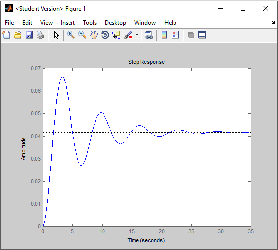
When the program execution completes a plot similar to the one shown above should appear. It is at this point that a visual analysis of the system may be done if desired. Should the code not execute or the plot looks different than expected, take another look at the code and compare it to the guide.