How to Make an Image Classification Model: Is It a Pie?
by Toufiq in Design > Software
442 Views, 2 Favorites, 0 Comments
How to Make an Image Classification Model: Is It a Pie?

Machine Learning/Deep Learning has found applications in numerous areas such as Computer Vision (Image Segmentation, Classification etc.), Natural Language Processing (Language Models; ChatGPT, Claude, etc.). In this instructables tutorial, we are going to make a Deep Learning Classification Model that we will train to classify pictures of food items; to tell whether it is a pie or not. For most machine learning/deep learning projects, the following workflow applies:
- Defining the problem to be solved (in a way that is relevant to machine learning).
- Gather and prepare the necessary dataset for solving the problem.
- Select and implement an appropriate machine learning model that suites the task.
- Train the machine learning model on the training data from the gathered dataset.
- Validate the model's performance using the validation data from the gathered dataset.
- Fine-tune the model if necessary.
Supplies

Not much is needed to pursue this project. Let's list the requirements.
- A working computer with internet access.
- Google Colaboratory
We are to use the Google Colaboratary online IDE as our programming environment, where we can load the dataset and train our model with free GPUs made available by Google.
It is also possible to build this project locally, but this is a much simpler route where we don't have to bother installing several libraries we may not often use.
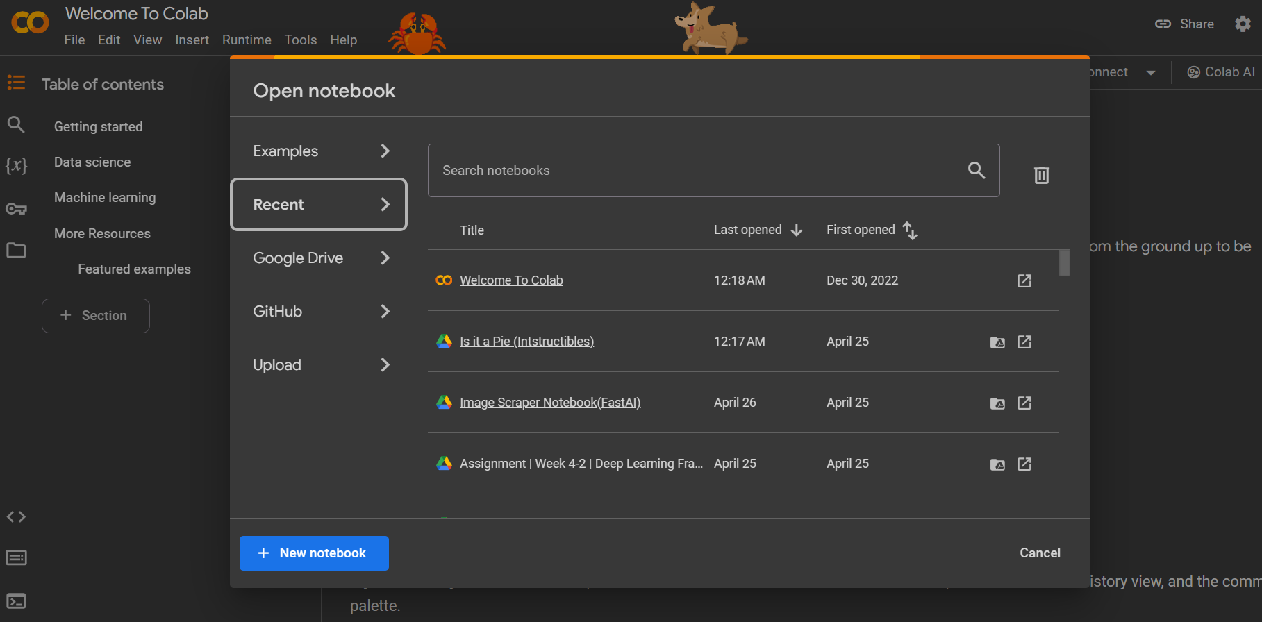
Let's start by opening Google Colaboratory, and creating a New Notebook.
Importing Libraries and Accessing the 'Is It a Pie?' Dataset
We will be importing the following libraries to use in this project.
#Image Loading and Viewing
import os
from PIL import Image
import matplotlib.pyplot as plt

#PyTorch Base Libraries
import torch
from torch import nn
from torch.utils.data import DataLoader, random_split

#PyTorch Computer Vision Libraries
import torchvision
from torchvision.utils import make_grid
from torchvision import datasets, transforms

device = torch.device('cuda' if torch.cuda.is_available() else 'cpu')
torch.__version__, device
We will continue by accessing the 'Is it a Pie?' dataset that was specially created for this tutorial. It is publicly available on the following Google Drive.
Dataset: https://drive.google.com/file/d/1G2QYobFcW1sn82Sirj79Eqewc3xUAO4t/view?usp=drive_link
All we will need from the link above to make access the dataset in our Notebook is the file ID (Between the 'file/' and '/view?' of the link).
File ID: 1G2QYobFcW1sn82Sirj79Eqewc3xUAO4t
In the first cell, we will write the first few lines of code to download and unzip our data.
!gdown -qq 1G2QYobFcW1sn82Sirj79Eqewc3xUAO4t # Downloading Dataset using the Google Drive File ID
!unzip -qq '/content/Is it Pie(Dataset).zip' # Unzipping the files

data_path = '/content/Is it Pie(Dataset)' # File Path to Dataset
The dataset folder consists of two subfolders, which represent the two dataset classes: 'Not a Pie', 'Yes, Pie'.
Loading Datasets and Viewing Some Images

We will first define a data transformation step that turns our data into the appropriate format for Deep Learning. (Psst.. I am referring to Tensors).
The transformations are then applied to the entire dataset. We applied augmentations to artificially inflate the amount of data that is used in training our final model.
# Data Transformation Step
data_transforms = transforms.Compose([transforms.CenterCrop(240), # Center Cropping Images
                                      transforms.Resize(size = (255, 255)), # Resize Images
                                      transforms.TrivialAugmentWide(num_magnitude_bins = 2), # Apply Augmentations
                                      transforms.RandomHorizontalFlip(p=0.7),
                                      transforms.ToTensor()]) # Convert Images to Tensors

# Applying Data Transforms to Entire Dataset
all_data = datasets.ImageFolder(root = data_path, transform = data_transforms)

# Creating a Temporary DataLoader to view all class images
all_data_loader = DataLoader(all_data, batch_size = 64, shuffle = True)
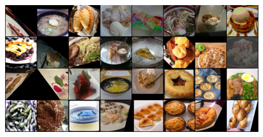
Let's view a sample of our entire dataset by loading a batch from the temporary DataLoader above. We use the imported <make_grid> module from torchvision, and the matplotlib library to display the samples, as written below.
images, labels = next(iter(all_data_loader)) # Load a Batch of Images
grid = make_grid(images[:32], normalize = True) # Create a Grid of 32 Image Samples
plt.imshow(grid.permute(1, 2, 0)) # Display the Images.
# Permute is Done to Make Tensors Viewable as Images
plt.axis('off')
We can now Split our original Dataset (all_data) into the training and validation DataLoaders for training our model. We use the imported random_split module to split our dataset in to 70% training set and 30% validation set.
batch_size = 64 # Number of Samples Learnt From Per Training Loop.

train_data, valid_data = random_split(all_data, [0.7, 0.3]) # Train-Test Split

train_dataloader = DataLoader(train_data, batch_size = batch_size)
valid_dataloader = DataLoader(valid_data, batch_size = batch_size)

classes = all_data.classes
classes
We are somewhat done with the data preparation step now.
Implementing an EfficientNet Model

It is possible that we can create a model from 'scratch' by defining how each and every single layer comes together. That may not be very optimal, since already existing model architectures which are pretrained with other datasets can learn and analyse our data much better.
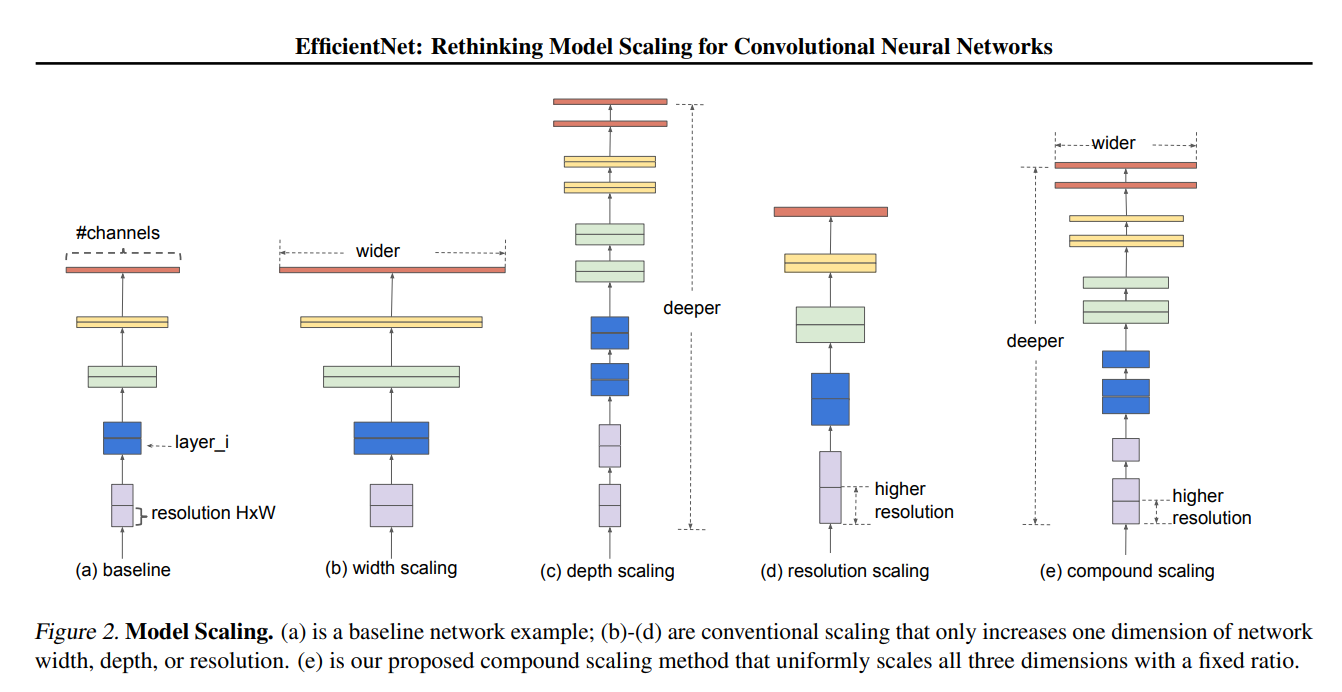
From the family of already existing models out there, we are going to use the EfficientNet architecture. EfficientNet achieves good results with reduced computational cost and model size. It uses a compound scaling method that uniformly scales all dimensions of the network (width, depth, and resolution) with a fixed ratio. It is efficient in terms of computation and memory usage.
We first load the pretrained weights of the model as follows.
weights = torchvision.models.EfficientNet_B1_Weights.DEFAULT # Loading B1 Variant Weights
weights
After loading the weights, we initialise the model with the pretrained weights.
model = torchvision.models.efficientnet_b1(weights = weights).to(device)
We can choose to freeze the layers of the model (model learns faster, but less accurate) ergo performing feature extraction, or not freeze the layers (model learns slower, could be more accurate) ergo performing fine-tuning. To freeze the layers, add the following.
for param in model.features.parameters():
  param.requires_grad = False
I choose not to freeze the layers.
We then edit the final layers of the model to fit our data. The Final Layer(Classifier Layer) of our model should have the same shape as the number of classes in our dataset.
output_shape = len(classes) # Number of Classes in Our Dataset


model.classifier = torch.nn.Sequential(
    torch.nn.Dropout(p = 0.2,inplace =True),
    torch.nn.Linear(in_features = 1280,
                    out_features = output_shape,
                    bias = True).to(device)
)
Model Training and Testing Loop
Instead of writing our model training and testing loop from scratch, we will use an already implemented one I adapted from LearnPytorch.io. Let's clone the git repository containing the implemented loops along with other helper functions, and import what we need from it.
!git clone -qq https://github.com/toufiqmusah/CALADAN.git # Cloning Repository
from CALADAN.modular_torch import engine, data_setup # Importing Needed Modules
Next, we setup our model hyperparameters (helps the model learn), and then the training loop using the <engine> module from the Repository.
criterion = nn.CrossEntropyLoss() # Loss Function
optimizer = torch.optim.Adam(model.parameters(), lr = 2e-3)
epochs = 20 # Number of Training Rounds

# Training Loop
model_result = engine.train(model = model,
                            train_dataloader = train_dataloader,
                            test_dataloader = valid_dataloader,
                            optimizer = optimizer,
                            loss_fn = criterion,
                            epochs = epochs,
                            device = device)
This should take a while to run. Ensure that the runtime type being used is GPU.
At the end of training, I ended up with a model having a training accuracy of [>95%], and a validation accuracy of [>85%].
Running Inference and Saving the Model

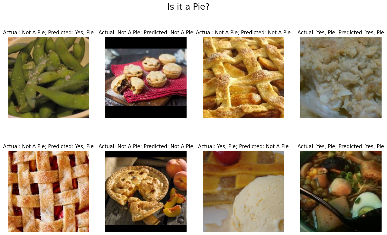
We run inference to test how well our model performs after training. We will use the following helper functions to run inference on several samples and display the results.
# Creating Testing Data
data_transforms = transforms.Compose([transforms.CenterCrop(240), # Center Cropping Images
                                      transforms.Resize(size = (255, 255)), # Resize Images
                                      transforms.ToTensor()]) # Convert Images to Tensors


# Applying Data Transforms to Entire Dataset
test_data = datasets.ImageFolder(root = data_path, transform = data_transforms)
test_loader = DataLoader(test_data, batch_size = 64)

model.eval() # Place Model in Evaluation Model

def predict(test_dl, model):
  for i, (imgs, targets) in enumerate(test_dl):
    imgs = imgs.to(device, dtype = torch.float)
    preds = model(imgs).detach()
    preds = torch.round(torch.sigmoid(preds)).flatten().to('cpu') #flatten output
    return imgs, preds, targets

imgs, preds, targets = predict(valid_dataloader, model)
We then plot the results as follows.
mapping = {0:'Not A Pie',1:'Yes, Pie'}

fig = plt.figure(figsize=(16,9))
for i in range(8):
  img = imgs[i].cpu() # send to cpu
  plt.subplot(2,4,i+1)
  plt.axis('off')
  plt.imshow(img.permute(1,2,0))
  plt.title(f'Actual: {mapping[targets[i].item()]}; Predicted: {mapping[preds[i].item()]}')
plt.suptitle("Is it a Pie?", fontsize=20)
plt.show()
To save and download our model:
from google.colab import files

torch.save(model, '/content/Is-it-a-Pie.pth')
files.download('/content/Is-it-a-Pie.pth')
Running Single Inference:
test_pie_path = '/content/Is it Pie(Dataset)/Yes, Pie/1112300.jpg'
test_pie = Image.open(test_pie_path)
test_pie = data_transforms(test_pie)
test_pie = test_pie.unsqueeze(0)
test_pie = test_pie.to(device, dtype = torch.float)
pred = model(test_pie).detach()
mapping = {0:'Not A Pie',1:'Yes, Pie'}
pred = torch.round(torch.sigmoid(pred))


if pred.tolist()[0][0] == 1:
   n = 0
else:
   n = 1

plt.title(f'Predicted: {mapping[n]}')
plt.imshow(test_pie.squeeze(0).permute(1, 2, 0).cpu())
plt.axis('off')
References
Project Notebook - Is it a Pie (Intstructibles) - Colab (google.com)
LearnPytorch - Zero to Mastery Learn PyTorch for Deep Learning
EfficientNet Paper - [1905.11946] EfficientNet: Rethinking Model Scaling for Convolutional Neural Networks (arxiv.org)