How to Make a Numerical Integration Program in Python
by RustySchackleford in Circuits > Assistive Tech
56453 Views, 8 Favorites, 0 Comments
How to Make a Numerical Integration Program in Python

This is a tutorial on how to create and run a program that will evaluate definite integrals using a numerical integration algorithm. I've divided the steps into 3 sections: understanding the algorithm that will be used to make the program, coding the program using the Python programming language, and running the program. This tutorial is intended for someone who may need to quickly make a calculator to evaluate definite integrals, or perhaps needs the algorithm for use in a larger scale program. Basic calculus knowledge is expected, but relevant mathematical information is reviewed. Knowledge of programming is not expected, but is useful since I only briefly describe how the programming actually works.
What you will need:
- A personal computer with access to the internet
Understanding the Algorithm Part 1: the Definite Integral and Its Use
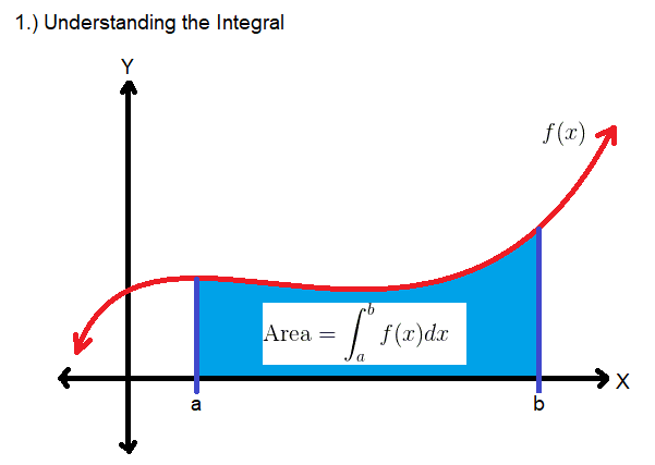
I will assume you know a little bit of what an integral is in the context of basic calculus. Integrals are important because they allow you to sum an array of values multiplied by an infinitesimal length; this is useful in many areas of finance, number theory, physics, chemistry, as well as many other fields. This program, however, will only allow you to calculate the area underneath a curve for a finite interval, or in other words, it does not evaluate anti-derivatives--a much more powerful algorithm is necessary for that. This algorithm is useful if you need to evaluate a definite integral in a larger program specified toward something else, or if you want to check your answer for any definite integrals done by hand.
A basic definite integral represents the area under a curve defined by a function e.g. f(x). For a definite integral, we seek the area between two points (labeled a and b respectively). In the picture, the turquoise region is the area I'm referring to, and the equation for determining this is also shown in that region. The function shown in the picture is arbitrary.
Understanding the Algorithm Part 2: Numerical Approximation
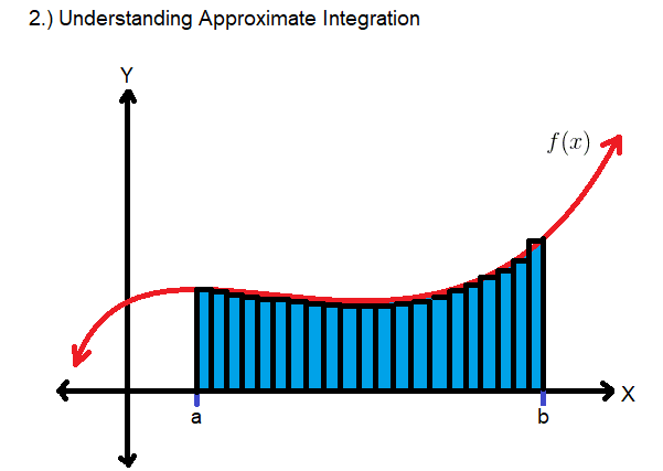
A computer needs a broad set of instructions for calculating that area underneath an arbitrary function that will work for any function, so analytical methods you may be familiar with are of no use since they are too particular. One method to compute integrals approximately, that a computer can actually handle, is done by filling the area of interest with a user-defined amount of rectangles of equal width and variable height then summing up all of the rectangle's areas. The rigid properties of rectangles will leave some of the total area untouched, hence why this is considered an approximation; however, the more rectangles you can cram in between the boundaries (a and b), the more accurate the approximation will be since the untouched regions become more sparse. Since a computer will be doing the task, you can set the number of rectangles in the desired region to be a very large number, making the approximation extremely accurate. In the supporting picture, imagine that each rectangle in the designated area is of equal width. I did my best to make them equal width in Microsoft Paint, but didn't do the best job.
Understanding the Algorithm Part 3: the Midpoint Rule
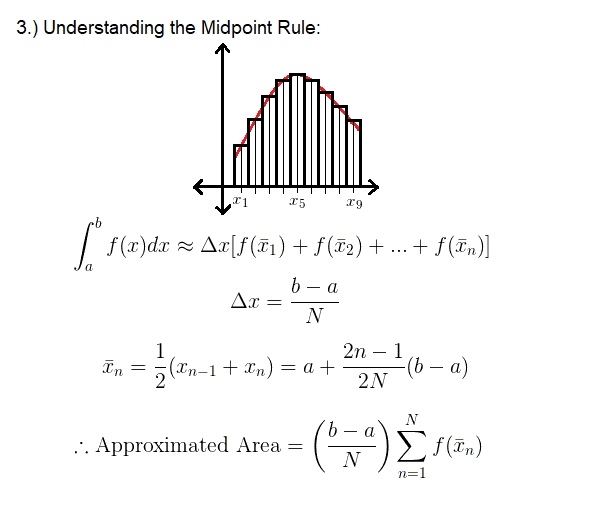
This rule designates how the rectangles are made and used in the approximation. Each rectangle out of "N" rectangles has to have an equal width, Δx, but each nth rectangle cannot be the exact same: the varying factor is the height which varies as the function evaluated at a certain point. The midpoint rule gets its name from the fact that you are evaluating the height of each rectangle as f(x_n), where "x_n" is the respective center-point of each rectangle, as apposed to the left or right of the rectangle. Using the midpoint is like implementing an average which will make the approximation more accurate than if you were to use the right or left. The supporting picture for this step summarizes how the midpoint rule is defined mathematically.
Creating the Program Part 1: Downloading a Python Compiler/Editor
Now that you understand the algorithm that needs to be implemented, it is a matter of getting a computer to perform the calculation for you. The first step to telling a computer what to do is getting the tools to do so. This algorithm can be coded in any language; for simplicity, this program will be coded in the Python language. To command your computer to perform operations with Python, you will need an editor that takes instructions written in that language that will then be compiled into machine language that your computer can understand so it can perform the tasks you tell it to do. In this day and age, an editor and compiler are usually integrated, however that is not always the case. You can use any editor/compiler you are comfortable with, but I will show you how to obtain my personal favorite for Python: Canopy. If you already have an editor/compiler, you can skip these steps.
- Go to https://www.enthought.com/product/canopy/
- Click Download Canopy
- Click the download button corresponding to your operating system
- The download will start automatically.
- Follow the instillation instructions after starting the execution file
- Run the Program
- Click "Editor" from the program main menu
- Click "create a new file" on the center of the screen
From this point you should see a blank white window with a cursor resembling a basic word processing document. You are now ready to start coding the numerical integration algorithm for solving definite integrals. The proceeding steps will have a snippet of code that you will copy and an explanation of what that snippet does for the program as a whole.
Creating the Program Part 2: Importing Functions & Defining Variables

Copy the code in the picture.
For any program you may find yourself coding, there will be variables. A variable is a name given to a value that will be operated on and that can change. In most programming languages (if not all) you have to initialize a variable before the program can make changes to it. In the case of this program I have named the variables "N," "a," and "b." These values represent the number of iterations ( AKA number of rectangles), lower boundary, and upper boundary respectively. You can name these anything you want, but to match the formulas given in "Understanding the Algorithm Part 3: The Midpoint Rule," it is best to keep them the same. Notice that they aren't just set to a specific value. This is because they are made inputs that, when the program is ran, the user of the program can define what the value will be. The text in quotes, after the input command, shows up when you run the program telling you what type of value to type in. You will also notice that "int" and "float" are used before the input designations. These terms tell the computer what type of variable this value will be. An "int" is an integer, and a "float" is a floating point value (i.e a decimal). It should be clear why these are designated as such.
Any text present after a "#" is a comment that allows the programmer to follow the code in a humanistic way; I have made certain comments in my code which you will be copying, but feel free to add any comments that help you specifically. The program will not read anything with a "#" before it as a command.
The portion of code that reads "from math import *" tells the program to import an array of mathematical functions that can be used without having to program them in yourself. The "*" just means "all." Read this portion of code as: from the math library import all of the functions. This allows you to use mathematical functions like sine, cosine, log, exp, etc. These function can be mathematically integrated within the code.
Creating the Program Part 3: Creating a Function for Integration

Copy the code in the picture below the previous code.
WARNING: This section is dense, and I want to clear some things up that could potentially be confusing. When talking about programming, the word "function" pops up a lot. This term also pops up a lot when you are talking about math. So, from this point on, when I'm talking about a function in the programming sense, I will write "Python function," and when I'm talking about the mathematical function, I will say "mathematical function." At some point we will use a Python function as a representation for the mathematical function in question.
This next snippet of code is the heart of the program. Here, a Python function is defined that carries out the algorithm of numerical integration using the midpoint rule. "def Integrate(N, a, b)" reads as: define a function called "Integrate" that accepts the variables "N," "a," and "b," and returns the area underneath the curve (the mathematical function) which is also defined within the "Integrate" Python function. You can call this Python function anything when you do the coding, but it makes sense to call it integrate since it is a function that indeed integrates a mathematical function.
At this point it is worth commenting on how Python segregates blocks of code. A block of code is an entire section that performs a certain task. Different programming languages will have designated ways to distinguish these "blocks." For Python, a block is distinguished by indentations: each task-performing-section has its own indent, and there can be indented blocks within other indented blocks. This represents tasks within tasks, and essentially tells the order in which the code needs to be executed. In the case of the defined Python function "Integrate," everything within that function is indented out one block thus distinguishing the tasks that will be executed within that function. There are indented parts within this Python function that perform their own tasks as well. It goes as follows: a command (task) is set forth, a colon follows the command, and what the command does is indented underneath.
Immediately after defining the "integrate" Python function, you will define another Python function called f(x). This represents the mathematical function that will be integrated. For each different mathematical function you want to integrate, you will have to take to this program line to change it (unlike the variables which are defined when the program is ran). Each Python function will have a return value, this is what the function returns when you throw it a value. In this case the thrown-in value is "x," and this "x" term will take the value of what ever you throw it--it is a temporary value.
Next, a for-loop acts as the summation defined in the formulas in the "Understanding the Algorithm" section of this tutorial. This summation requires a couple more variables, one of which will act as the return value for the entire "Integrate" Python function. Before the for-loop, I have designated these variables as "value," and "value2." the task of the for-loop is to iterate over a range of values for a designated variable, which can conveniently be defined within the for-loop command; in this case, that variable is "n." The range for which the iteration occurs is 1 to N+1. You should notice that the summation defined in the aforementioned formulas only ranges from 1 to N. We define it this way because the Python language counts each iterated value starting from zero, so we essentially have to shift the range of the values to fit our desired range. The for-loop then allows for the summation of all of the rectangle's heights together and stores that value into the variable which I called "value." This is seen in the piece of code that shows up as: value += f(a+((n-(1/2))*((b-a)/N))).
From there, the next piece of the code utilizes the variable called "value2" which is then assigned to be the sum of all of the heights of each rectangle multiplied by the standardized width of each rectangle--this is our final answer that we want displayed by our program, and is thus the return value of the "Integrate" Python function.
Creating the Program Part 4: Displaying the Answer

Copy the code in the picture below the previous code.
Now that the answer can be obtained through the "Integrate" Python function, we want to be able to display it. This is just a matter of putting the values that were input by the user ("N," "a," and "b") into the "Integrate" Python function and printing it on the screen. This command is shown on line 21, and is really all that you need to do to finish this step. The code on lines 19 and 20 are just there to "pretty up" the output of the entire program. "print("............................")" separates the input section of the program from the output section, and "print("Here is your answer: ")" is just a designation that the answer will be printed after that line of text.
Running the Program Part 1: Running the Program As Is
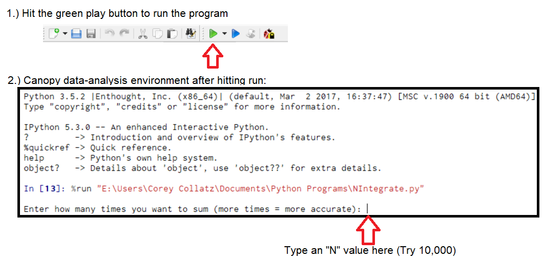
If you're not using Canopy, then you probably don't even need to follow this step at all and running the program may require different procedures. In Canopy, before you are able to run the program, you will need to save it. The file type for a Python program is a .py file--it automatically saves as this. Pick where you want the file to be saved, then you will be able to run the program.
Running the Program:
- Hit the green button that looks like a "play button" located on the tool bar just above where your file name shows up (refer to picture).
- The program will then run in the bottom screen of the editor which is known as the Canopy data-analysis environment. Assuming you copied the prompts as I wrote them, you should see at the bottom of the Canopy data-analysis environment the prompt: "Enter how many times you want to sum (more times = more accurate): ." (refer to picture)
- Enter in a value for how many times you want to do the iteration i.e 10000 (how many rectangles you want to shove into your area), then hit enter.
- More prompts will appear with statements that should be the familiar input prompts you coded into the program in step 5. Fill them out appropriately just as in number 3 above.
- The integral should be evaluated, and a result should appear.
If you coded the program as shown in the preceding pictures, you have just integrated f(x) = x^2 over some bounds. The integral of x^2 is an easy to evaluate by hand, therefore you should check and make sure the program gave a very close answer to the correct analytical value determined by hand. When I run the program with the values N = 10000, a = 0, and b = 10, I get the answer 333.33333249999964. The correct analytical answer, is 333.333. This is incredibly accurate and quick. You have essentially squeezed 10,000 rectangles between 0 and 10 on the x axis and used them to approximate the area under the curve x^2!
Running the Program Part 2: Integrating Other Mathematical Functions
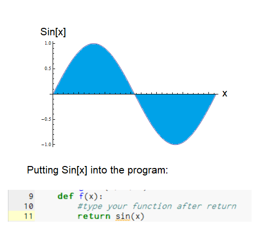
In the previous step, if you have been following along faithfully, you integrated f(x) = x^2. That is not the only mathematical function this program can integrate. Recall from step 5 you imported the math library array of Python functions into the program. This allows you to use more complicated mathematical functions that can be integrated. Let's give one a shot. Of course, you can use any function you'd like, but I'll further demonstrate the accurateness of this code by integrating a particular mathematical function that yields a well known value when integrated over a certain range. That function is f(x) = Sin[x]. This mathematical function is displayed in the first accompanying picture, plotted from 0 to 2π, and the area of interest is shaded in turquoise. There is an equal amount of positive area as there is negative area in this interval, so if you add up the total area, you should get zero. Let's see if this actually happens:
Putting the mathematical function f(x) = Sin[x] into the program:
- Before running the program again, under the comment "#type your function after return," type: sin(x) where x**2 is currently located. (refer to picture).
- Run the program by hitting the green play button again.
- Type 10000 for the N value (how many times you want to sum).
- put "0" in for the lower boundary.
- Put 6.2832 in for the upper boundary (approximately 2π).
- See what value you get.
When I did this, I ended up getting a value of 1.079e-10: this equates to .0000000001079, which is really close to zero, so it does appear to be accurate, and shows that the algorithm adequately handles negative area.
Running the Program Part 3: Expanding the Program
At this point you are done: you have a working definite integral algorithm coded up in Python that runs smoothly and gives very accurate answers. However, this program can be improved. I am not a programmer, and I have minimal experience with Python. In fact, I had to refresh myself on using Python to complete this tutorial, but that should give you confidence that Python is such an easy language to learn. My point is that you can expand on this program by making it more efficient, maybe implement some GUI, and make it more user friendly.
My thoughts on expanding the program:
- Implement a graphic user interface that allows you to run the program without using the Canopy interactive data-analysis environment
- Make it so that the mathematical function to be integrated doesn't have to be input inside of the program, but can be input after the program is ran (I was initially trying to do this, but couldn't figure it out).
- Define an "Integrate" Python function so it takes the f(x) function as apposed to having the f(x) function defined within it.
These are just some examples of areas of improvement, but I guarantee there are many other areas it can be enhanced. So I leave this step as an example of the flaws this program has and perhaps an exercise to anyone who wants to improve the program further.