How to Create a Simple Database on Excel Using Filters
by JacobD22 in Circuits > Microsoft
3228 Views, 16 Favorites, 0 Comments
How to Create a Simple Database on Excel Using Filters
List of steps:
Step 1: Two options to Import data
(1.1) Using Copy and Paste
OR
(1.2) Importing Data from a file
Step 2: Implementing the Lookup function
(2.1) Setting up the lookup() function
(2.2) IMPORTANT: Sort the data in order for proper results
Step 3: Filtering data using the data Filter
(3.1) Setting up the filter
(3.2) Numeric style filters
(3.3) Alphabetic style filters
Step 4: Incorporating graphs with filters
Step 5: Putting it all together
This can be done on any computer equipped with Microsoft Excel from 2007 onward. This Instructable assumes that you have a basic working knowledge of Excel such as typing data into cells and navigating the command bar.
(1.1) Importing Data Into Excel by Copying and Pasting
There are two options when importing data into Excel. This copy and paste method is useful for a broad range of data. The second (explained in section (1.2) is useful for importing massive amounts of data.
The steps to copy data can be used for data tables found on the internet, other excel files, and notepad files.
Simply click the left mouse button button down to start selecting data
Drag the mouse cursor while holding the mouse button down and release the mouse button
The cells that you have selected should be highlighted with a grey color and surrounded by a thicker border
Please note that the initial cell you clicked on will be white
Once you have selected the data, right click and select Copy, or you can use the Ctrl + C keyboard shortcut
Now, move to your Excel spreadsheet and paste the data by right clicking and selecting Paste, or using
Ctrl + V
(1.2.1) Importing Data From a File
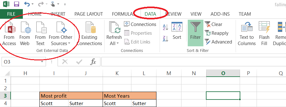
The second option utilizes a feature that is located in the Data tab on the toolbar
There are 4 options from which you can choose to import data:
From Access - Import data from Microsoft Access
From Web - Import data from a website
From Text - Import data from .CSV files and .TXT files
From Other Source - Lists other sources
(1.2.2) Importing Data From a Text or CSV File
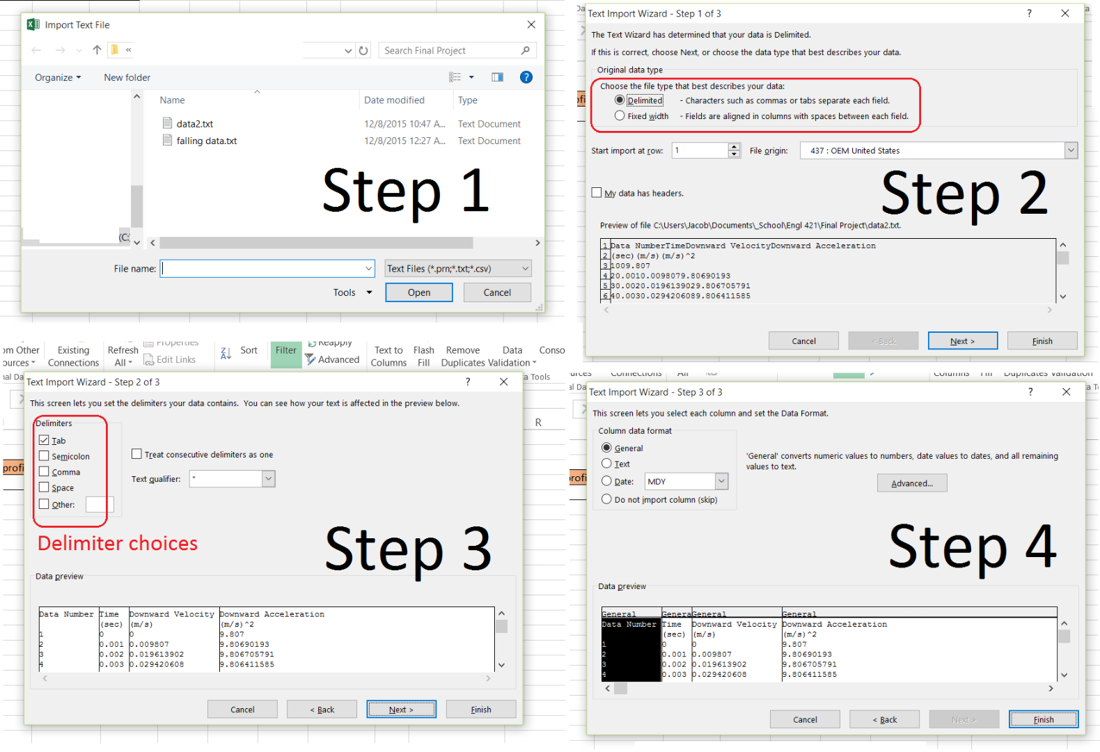
The most commonly used import method is the import from text method.
Step 1) When you click on the From Text icon a dialogue box will pop up asking for the file to be imported.
Step 2) After choosing the file, the text import wizard will pop up allowing you to choose options
- It is important to choose delimited for most situations as that gives you more control over how the data is imported.
- Delimiters are commas, periods, or spaces that separate the individual data points in the text file that the computer uses to separate different columns of data
Step 3) The next step of the wizard allows you to choose delimiters and will show you a preview of the data
Step 4) The wizard then allows you to choose whether you would like the data to be imported as numbers or as text
(2.1) Incorporating the Lookup Function
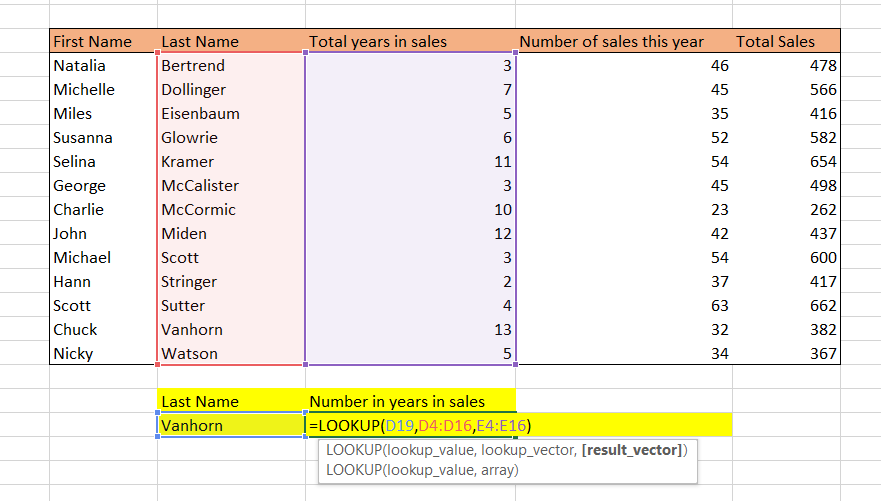
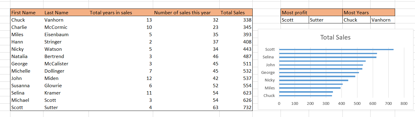
Suppose you wish to find the amount of sales that an employee has made for a current year.This can be done using a very handy tool called the Lookup function.
The lookup function can be selected from the Lookup and Reference tab under the function toolbar, or by typing = LOOKUP(lookup_value, lookup_vector, [result_vector]) in a cell.
The lookup_value is the number or text that you wish to search for.
The lookup_vector is the vector (set of cells) in which the function will try to find the input number or text.
The result_vector is the vector (set of cells) in which the lookup function will choose an output
For the above figure, the lookup value is Vanhorn, the lookup vector is the Last Name column, and the result vector is the Total Years in sales column.
MAKE SURE TO FOLLOW STEP 2.2 OTHERWISE THE LOOKUP FUNCTION MAY NOT WORK
For more information on the lookup function, Microsoft Office has detailed documentation on its support website and by searching for lookup. https://support.office.com/
(2.2) Organizing the Data
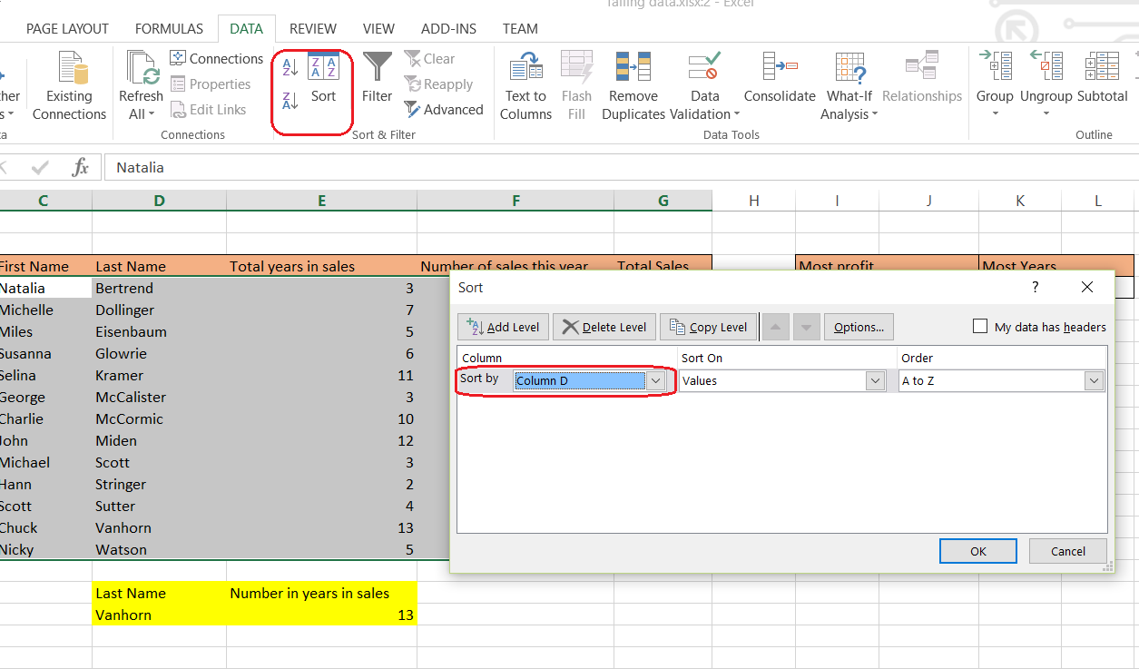
Unfortunately the lookup function can only be used when the cells that are part of the lookup vector are sorted.
To sort the cells, select all of the data in the table. (Refer to step 1 for help on selecting multiple cells)
Underneath the data tab, click on the sort icon. An input box will appear.
Choose the column where the lookup_vector is located. Then choose largest to smallest for numerical values or A to Z for text values. Press OK when you are ready to sort.
(3.1) Using the Filter
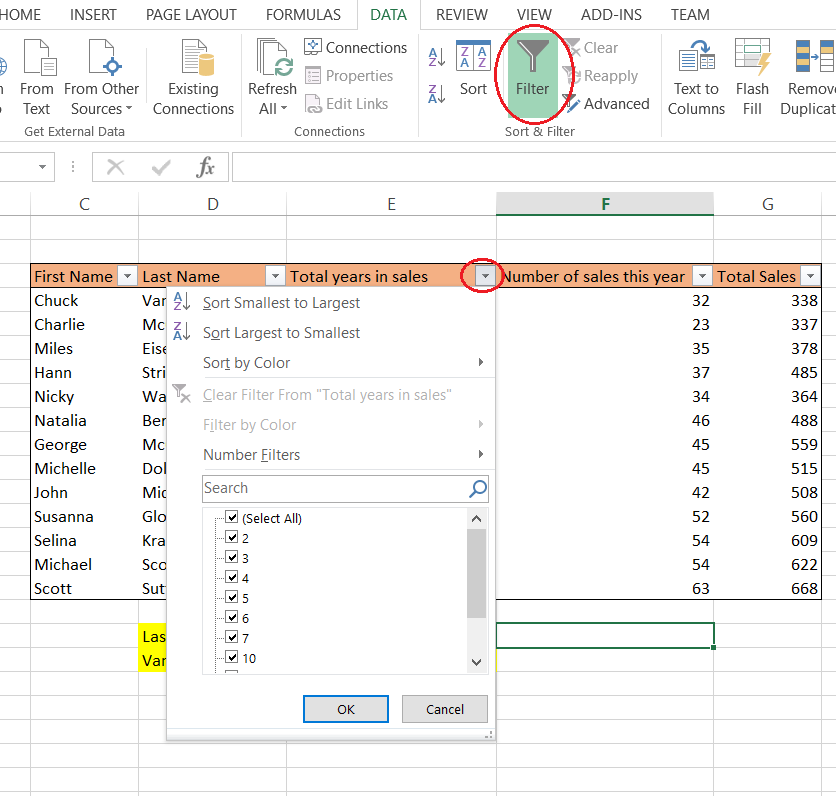
The Filter can be used to sort data, is able to search for specific queries, and can be used to filter out certain data ranges, allowing users to view important data from a large amount of information.
To use a filter select all of the data click on the Filter icon underneath the data tab.
A button with a triangle will appear on top row of the data in each column.When this is clicked a drop-down menu appears with sorting and filtering options along with a search bar.
Unfortunately filters can only be used once per page in Excel
To remove a filter entirely, click on the same icon that you used to create the filter, the green background of the icon and the drop-down triangles should disappear.
If you wish to remove a specific filter, click on the drop-down menu and click Clear filter from ..... This will set the data back to normal.
NOTE: Filters do not remove the data. Instead, they hide the Entire Row that holds data that is being filtered. If Susanna's name was filtered, the entire row holding her name, sales, and other information would disappear.
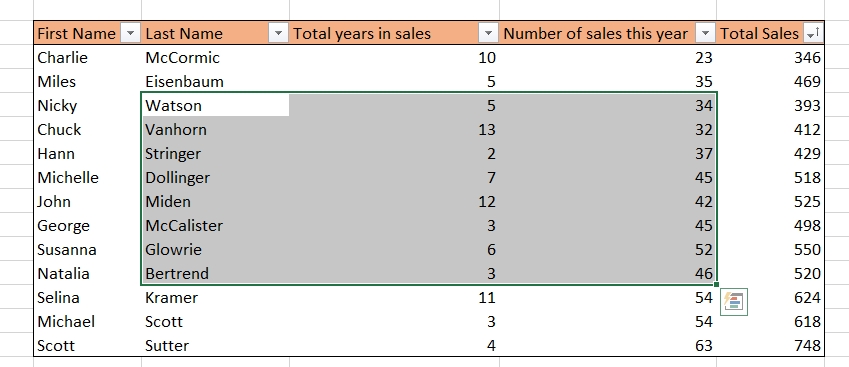
(3.2) Utilizing Numeric Filters
The numeric filters can filter out data with specific conditions:
To set up a numeric filter click on number filters from the drop-down menu.
Choose one of the filter types outlined in the menu
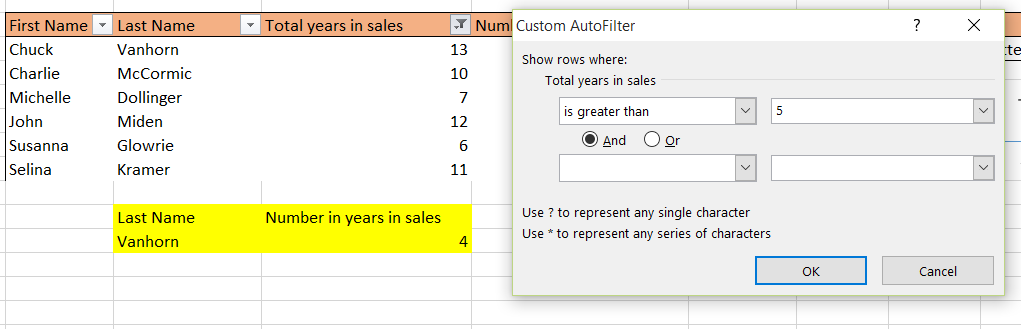
Numerical comparisons such as greater than, less than, or between two numbers can be used. It can also filter if the data is equal to or not equal to a certain number, and a custom filter can be set up to filter two conditions simultaneously.
For instance, the figure above shows all workers who have worked more than 5 years or less than 3 years and filters out the rest.
(3.3) Utilizing Alphabetical Filters
The Alphabetical filters allow a wide range of customization.
To create a filter that can search for peoples names that begin with a certain letter, click on the drop-down menu, click on text filters, and then click on the Begins With option.
Input your letter, or even a set of letters into the dialogue box that pops up and then press Ok.
The above figure was created using a begins with filter with an input of Ch.
(4) Creating Graphs of Functions
To insert a graph into your spreadsheet, select the data you wish to graph and click on the graph icon you wish to use in the charts area on the Insert tab.
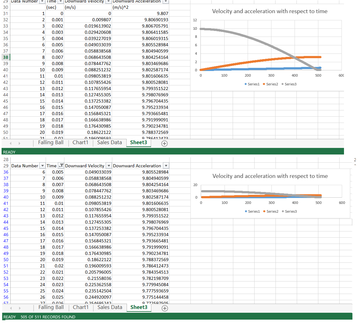
The chart will continue to display the data in the table that has not been filtered out. However, move the graph above the table as it may disappear when the table is filtered.
If the graph disappears, remove the filter and the graph should reappear. Also note that graphs that are inserted after the filter is used will "disappear" when the filter is taken off. The graph is in the same row as it was previously which may mean that if there was a lot of data filtered out, the graph is farther down in the spreadsheet.
If you look at the figure above, the first image shows a graph that is sized appropriately, while the second shows the effects of a filter that removed rows 1 through 5 from the data table. The graph is smaller as the rows in between the top and bottom are hidden. If the filter were to filter out rows 1 to 15, the graph would disappear completely.
(5) Putting It All Together
The great thing is that Filters can be used consecutively with the lookup() function.
This means that instead of manually sorting (step 2.2) sorting only takes two clicks. To sort the data, select the drop-down menu for the column you need to sort (remember from least to greatest).
The lookup() function will operate in a similar manner, but caution will be needed to create a proper lookup table. As the filter does not sort data that is hidden, simply remove the filter, sort the data, and then apply the filter again to allow the lookup() function to operate correctly.
You can successfully make a simple yet powerful Excel database by using the filter and lookup() functions. Information on how to create charts and graphs in Excel can also be found on the Microsoft Office support website.