How to Create a College-Style Budget Using Excel
by jkirkland1954 in Circuits > Microsoft
38560 Views, 30 Favorites, 0 Comments
How to Create a College-Style Budget Using Excel
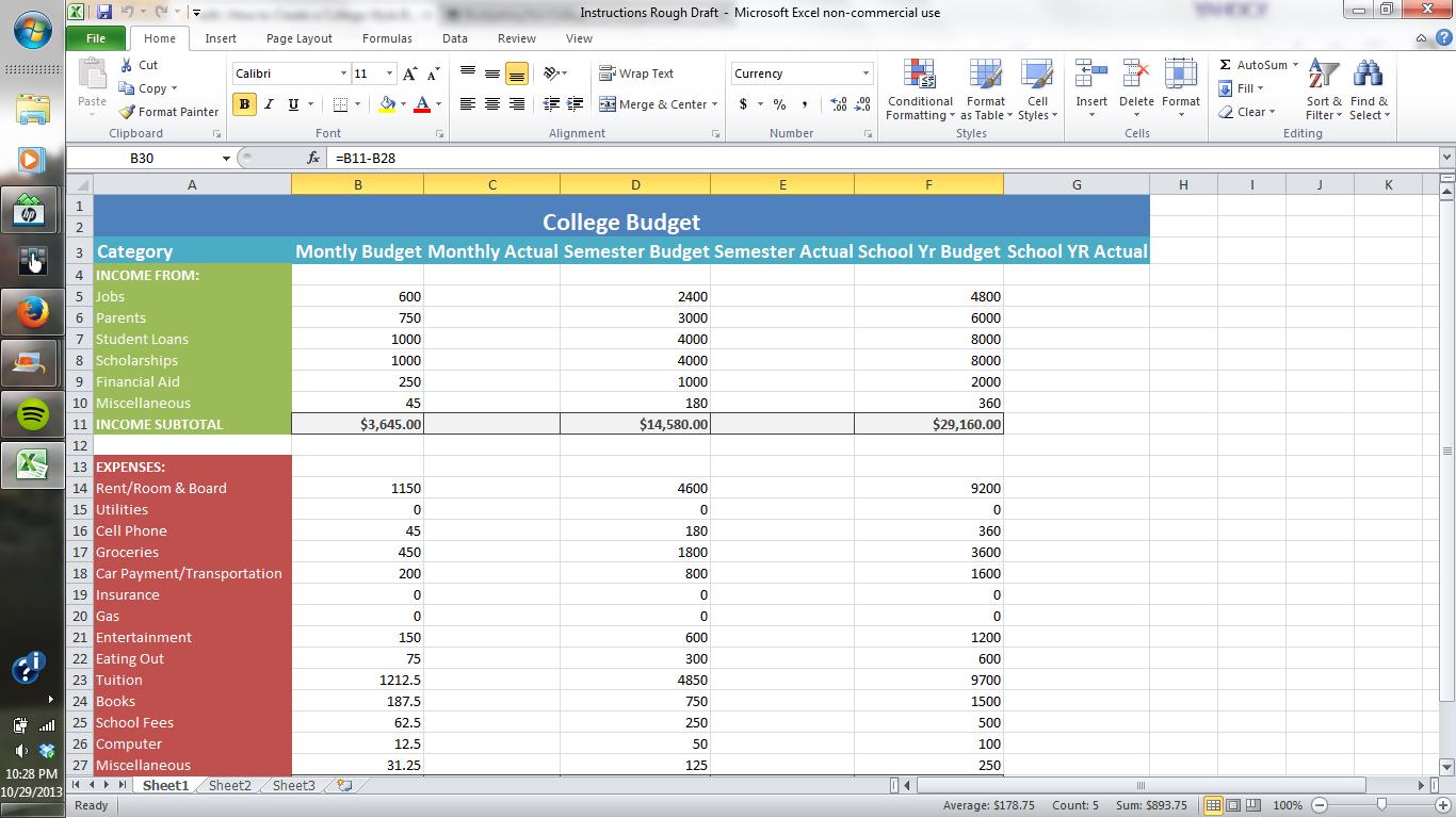
Microsoft Excel is a very powerful tool that is used in the business world everyday. Most often it is used to communicate how a business is performing financially, but its’ uses are endless. Whether your using Excel to create a complicated Profit and Loss Statement or a simple monthly budget, it can make working with numbers a little easier. As an employer or an employee, having the ability to effectively use Excel is a very important skill to obtain. By going through this Instructable you will learn the fundamental names and commands in Excel and how to use these basic skills to create a monthly budget.
Basic Functions of Excel Video
Create Title


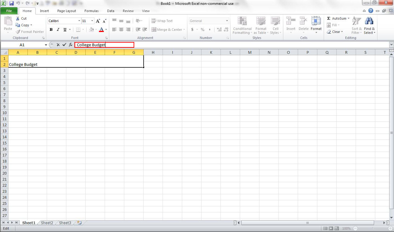
I. Start by selecting cells in A1-G2
II. Next, click “Merge & Center” on the toolbar. This will turn the previous selection into a new, single cell.
III. Now, enter the text in the newly formed cell by clicking on the formula bar.
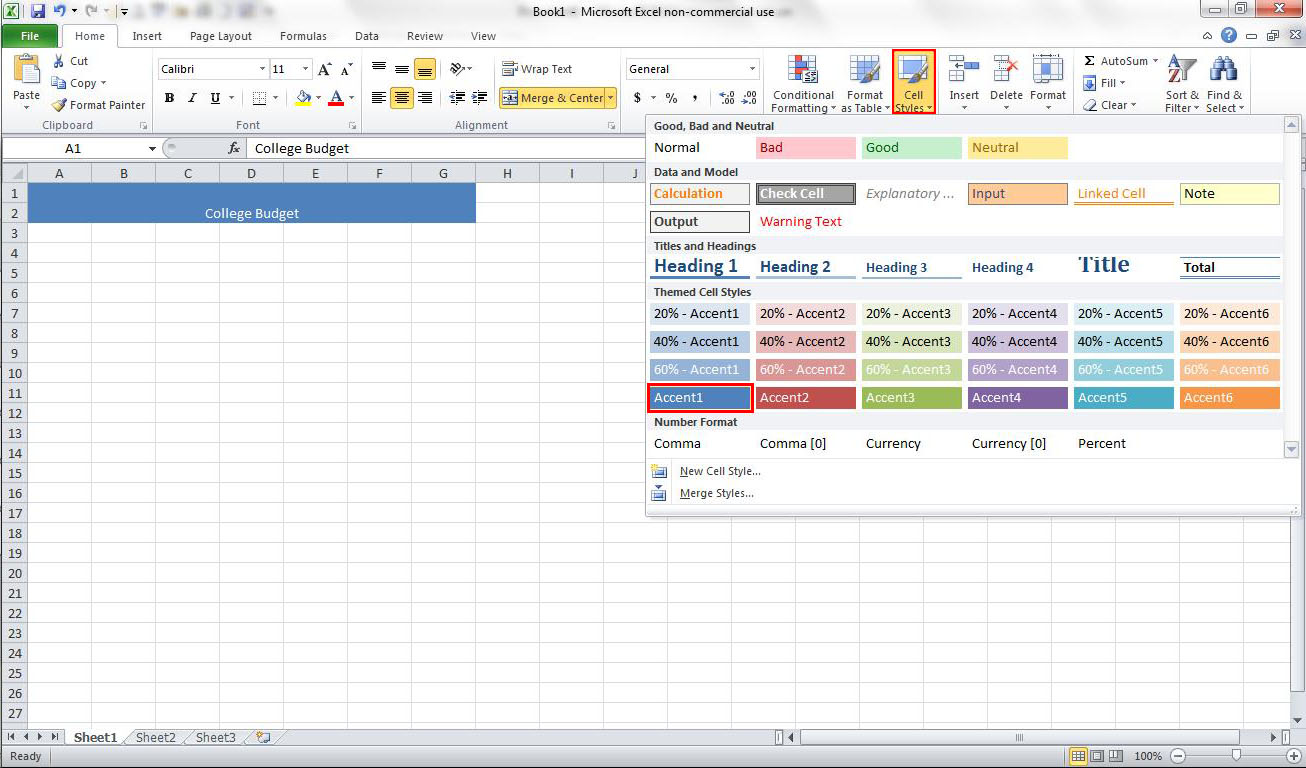
IV. The final part of this first step is to format the title. First, select the cell and then click on “Cell Styles” on the tool bar, and select “Accent 1.” Finally, change the font size to 16.
Create Column Headings
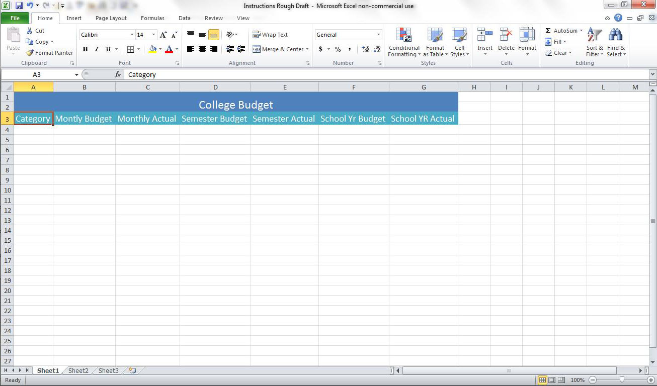
I. Start by selecting cell A3 and entering “Category” in it. Continue across the row by adding:
o “Monthly Budget” to B3
o “Monthly Actual” to C3
o “Semester Budget” to D3
o “Semester Actual” to E3
o “School YR Budget” to F3
o “School YR Actual” to G3
II. The next part is to format A3-G3 by selecting all cells and clicking on “Cell Styles” in the toolbar and choosing “Accent 5.” Set the font to 14 across A3-G3.
III. Lastly Autofit all columns (Refer to Intro Video for instructions on how to do this).
Create Row Headings for Income
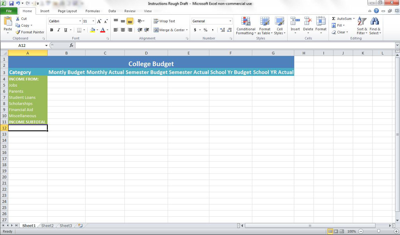
I. Select cell A4 and enter “INCOME FROM.” Continue down the Column by entering the following:
o “Jobs” in A5
o “Parents” in A6
o “Student Loans” in A7
o “Scholarships” in A8
o “Financial Aid” in A9
o “Miscellaneous” in A10
o “INCOME SUBTOTAL” in A11
II. Next, select cells A4-A11. Click on “Cell Styles” in the toolbar and choose “Accent 3.”
III. Finally, select cell A4 and make the font bold-faced; do the same for A11. Autofit Column A.
Create Row Headings
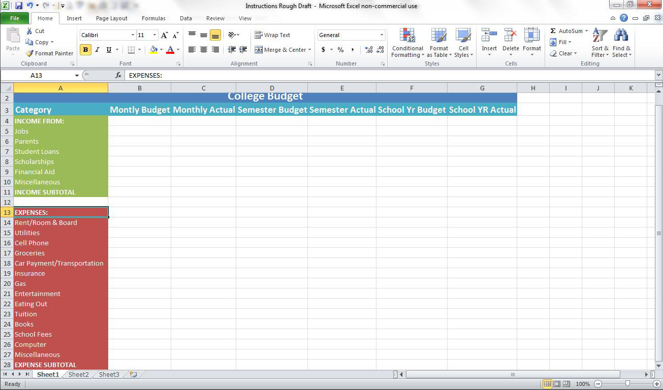
I. Select cell A13 and enter “Expenses:” continue down the column by adding:
o “Rent/Room & Board” to A14
o “Utilities” to A15
o “Cellphone” to A16
o “Groceries” to A17
o “Transportation” to A18
o “Insurance” to A19
o “Gas” to A20
o “Entertainment” to A21
o “Eating out” to A22
o “Tuition” to A23
o “Books” to A24
o “School Fees” to A25
o “Computer” to A26
o “Miscellaneous” to A27
o “EXPENSE SUBTOTAL” to A28
II. Select cells A13-A28 and click on “Cell Styles” in the toolbar. Choose “Accent 2.” Select cell A13 and make the font bold-faced, do the same for A28. AutoFit Column A.
Create Row Heading for Net Income
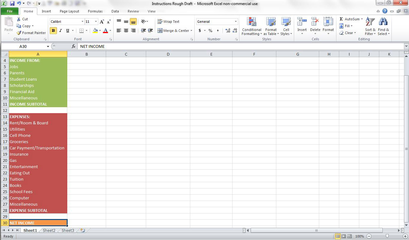
I. Begin by selecting cell A30 and enter “NET INCOME.”
II. Next, with cell A30 still selected, click on “Cell Styles” in the toolbar and choose “Accent 6.”
III. Make the font in this cell bold-faced.
II. Next, with cell A30 still selected, click on “Cell Styles” in the toolbar and choose “Accent 6.”
III. Make the font in this cell bold-faced.
Fill Income Categories
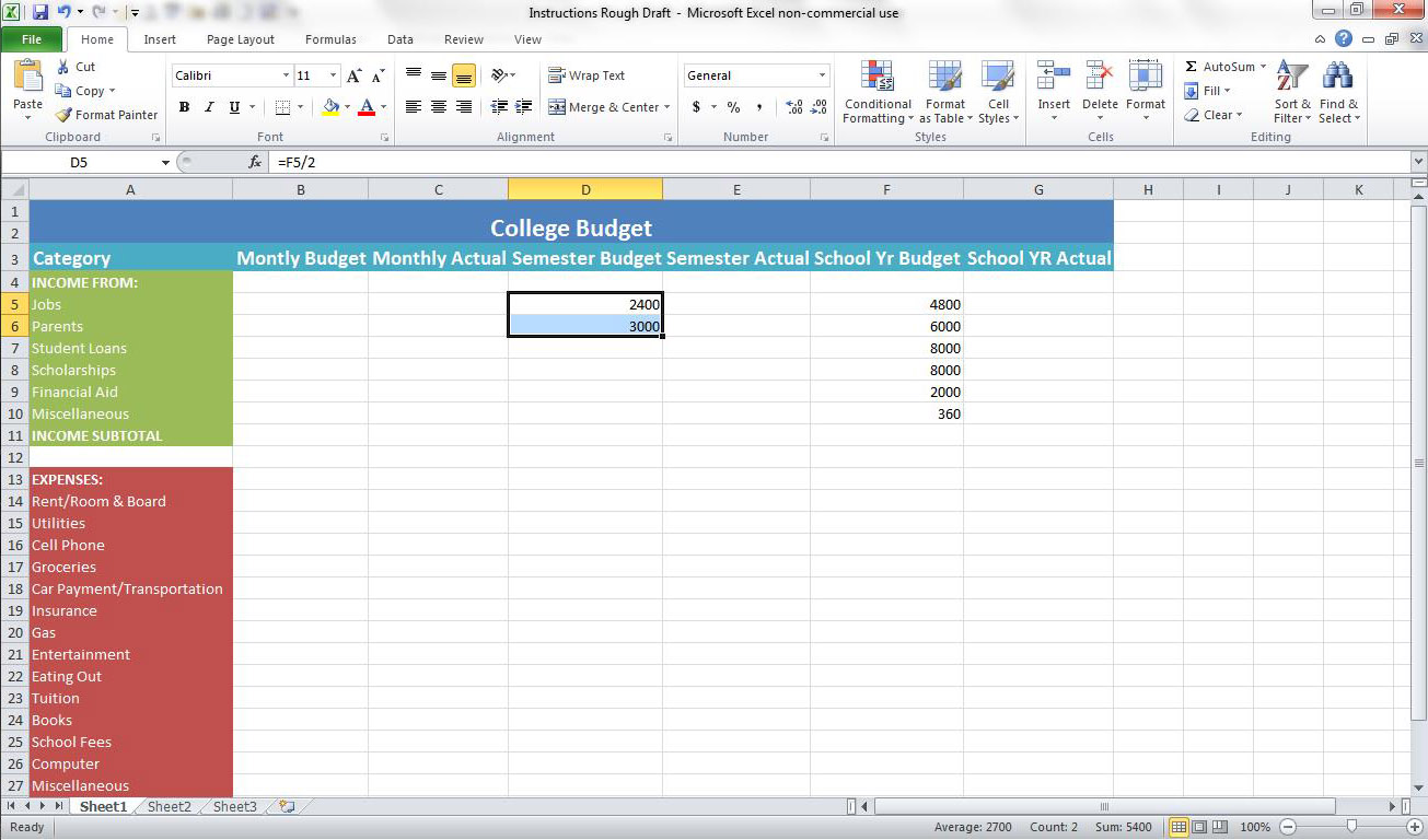
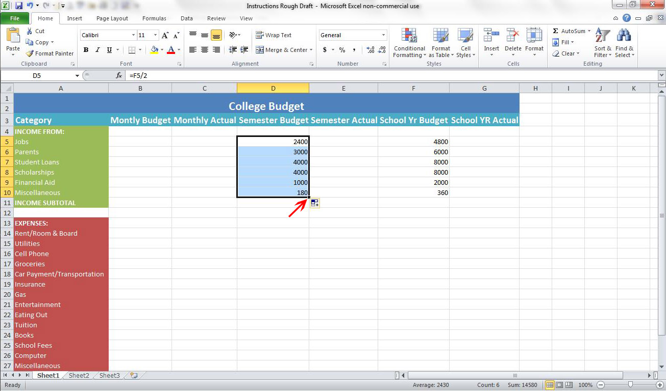
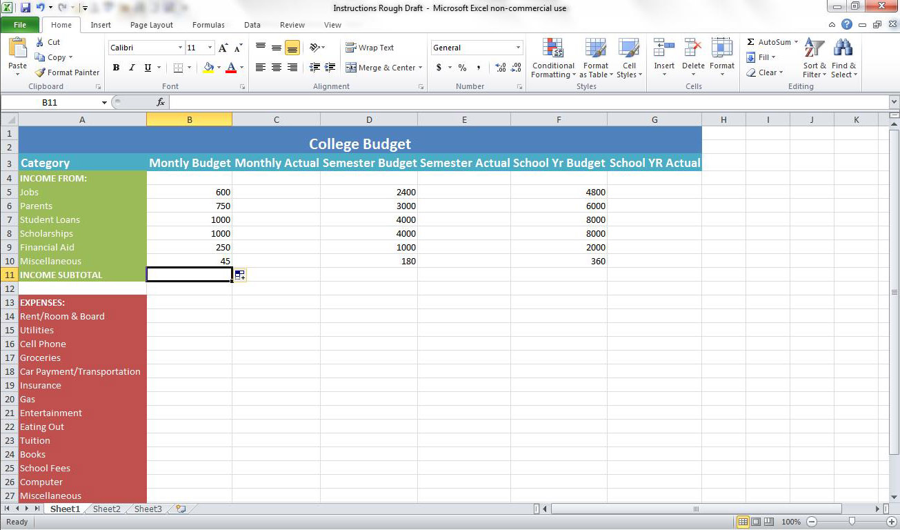
I. Begin by selecting cell F5 and enter the amount of income received from jobs. (Note: the numbers used in this budget are based on amounts determined to be average by the University of Tennessee-Knoxville. You will obviously choose numbers that reflect your personal income categories.) For this example we will enter the following numbers into the corresponding cells:
o “4800” in F5
o “6000” in F6
o “8000” in F7
o “8000” in F8
o “2000” in F9
o “360” in F10
II. Next, select cell D5 and enter “=F5/2” this will give us the appropriate amount for the semester since, in this case, a school year consists of two semesters. After this, select cell D6 and enter “=F6/2” and hit the enter key. Select cells F5 and F6 and hold the cursor over the bottom left corner of cell F6 until the cursor becomes a black plus sign, as shown in the figure below.
III. Click on the bottom right corner where the cursor has become a black plus sign (this appears when holding your cursor over the bottom right corner of D6 while both D5 and D6 are selected) and drag it down through cell D10. This will automatically fill cells D7-D10 with the correct formula, hence saving time.
IV. The process for filling in the Monthly Budget Income Categories is essentially the same as it was for the Semester Budget Income Categories. To begin, select cell B5 and enter “=F5/8” (Note: For this budget we have assumed that a semester is four months long, thus a two-semester school year would consist of 8 months). Select cell B6 and enter “=F6/8” then select cells F5 and F6. Use the AutoFill feature mentioned earlier to fill in cells F7-F10.
Fill Expense Categories
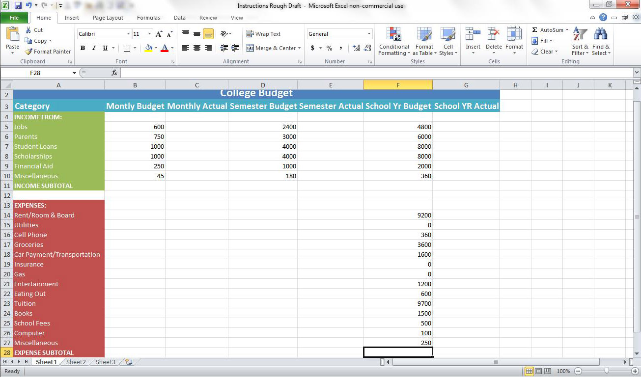
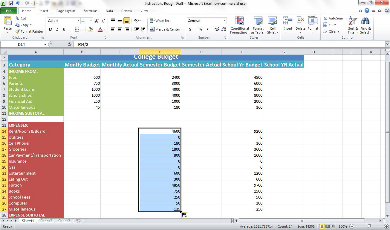
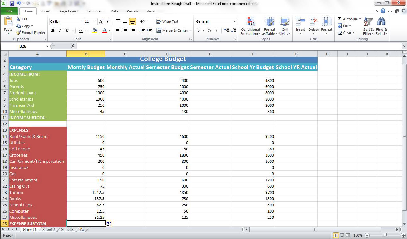
I. Select cell F14 and enter “9200” (Note: For this example we have chosen to use the estimates provided on the University of Tennessee-Knoxville website.) Next, fill in cells F15-F27 in the same manner. The following values are used in this example:
o “0” for F15
o “360” for F16
o “3600” for F17
o “1600” for F18
o “0” for F19
o “0” for F20
o “1200” for F21
o “600” for F22
o “9700” for F23
o “1500” for F24
o “500” for F25
o “100” for F26
o “250” for F27
II. Continue by selecting cell D14 and enter the formula “=F14/2” then select cell D15 and enter “=F15/2”. Autofill the cells D16-D27 by selecting cells D14 and D15 and dragging the black plus sign (this appears when holding your cursor over the bottom right corner of D15 while both D14 and D15 are selected) from D15 from D27.
III. Next, click on cell B14 and enter “=F14/8” hit the enter key once to select cell B15 and type “=F15/8” into this cell and hit enter again after keying that entry. Select both B14 and B15 and Autofill the cells F16-F27.
Determine Subtotals
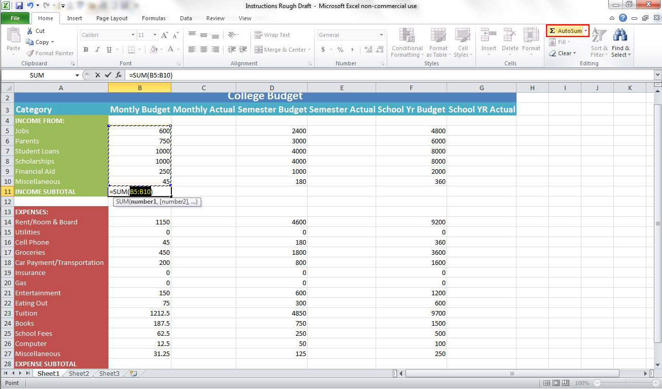
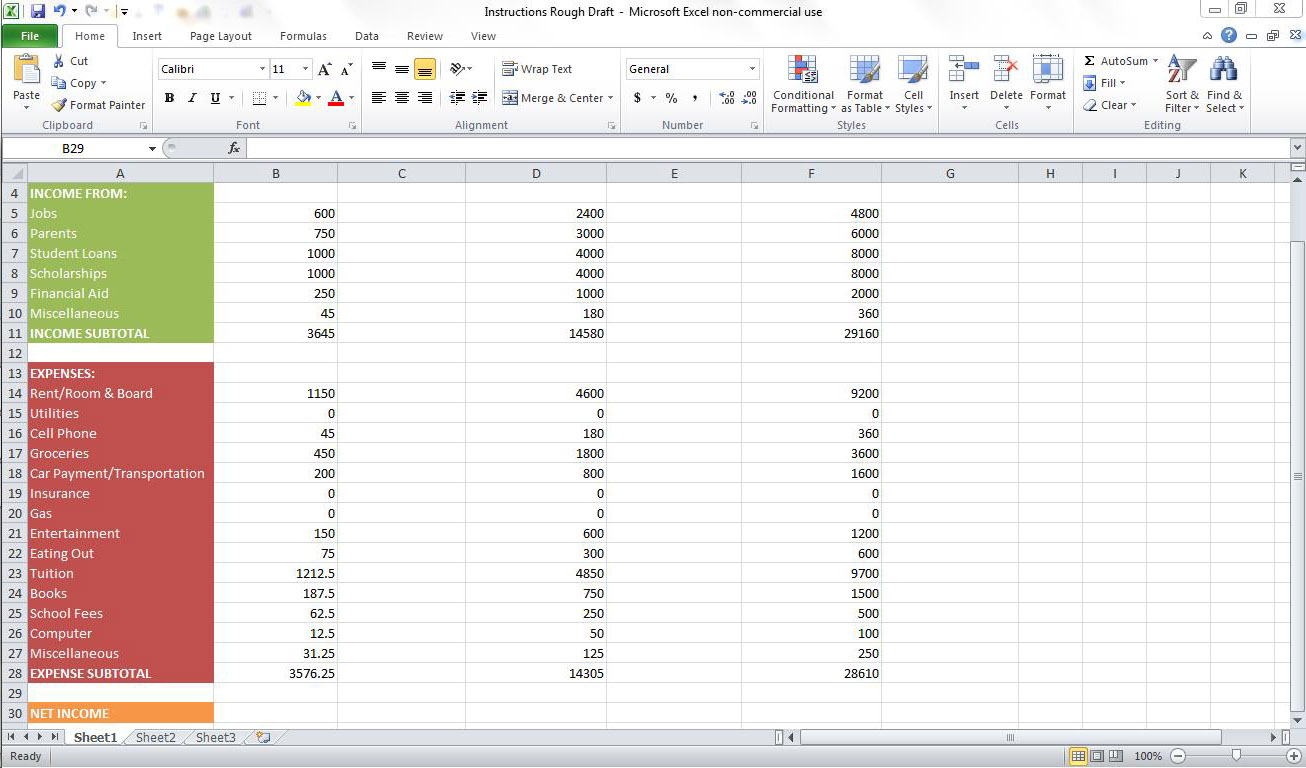
I. To determine the subtotals in each category, the AutoSum feature on the toolbar will be used. Start by selecting cell B11 and then clicking on the AutoSum feature located near the top right corner of the tool bar. The following should appear in cell B11: “=SUM(B5:B10)” Hit enter once this appears and the correct value will appear.
II. Repeat the process for cells D11, F11, B28, D28, F28.
II. Repeat the process for cells D11, F11, B28, D28, F28.
Format Subtotals
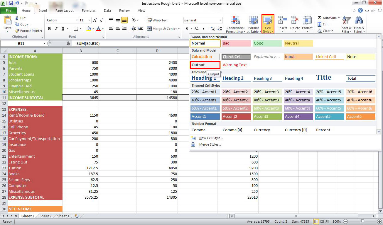
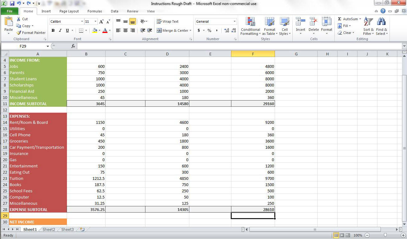
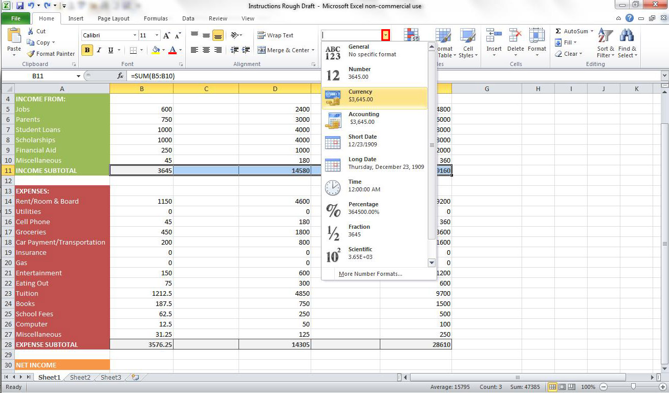
I. Begin by selecting cells B11-F11 and then click on “Cell Styles” and choose “Output”.
II. Repeat this process for cells B28-F28 in the Expense Section.
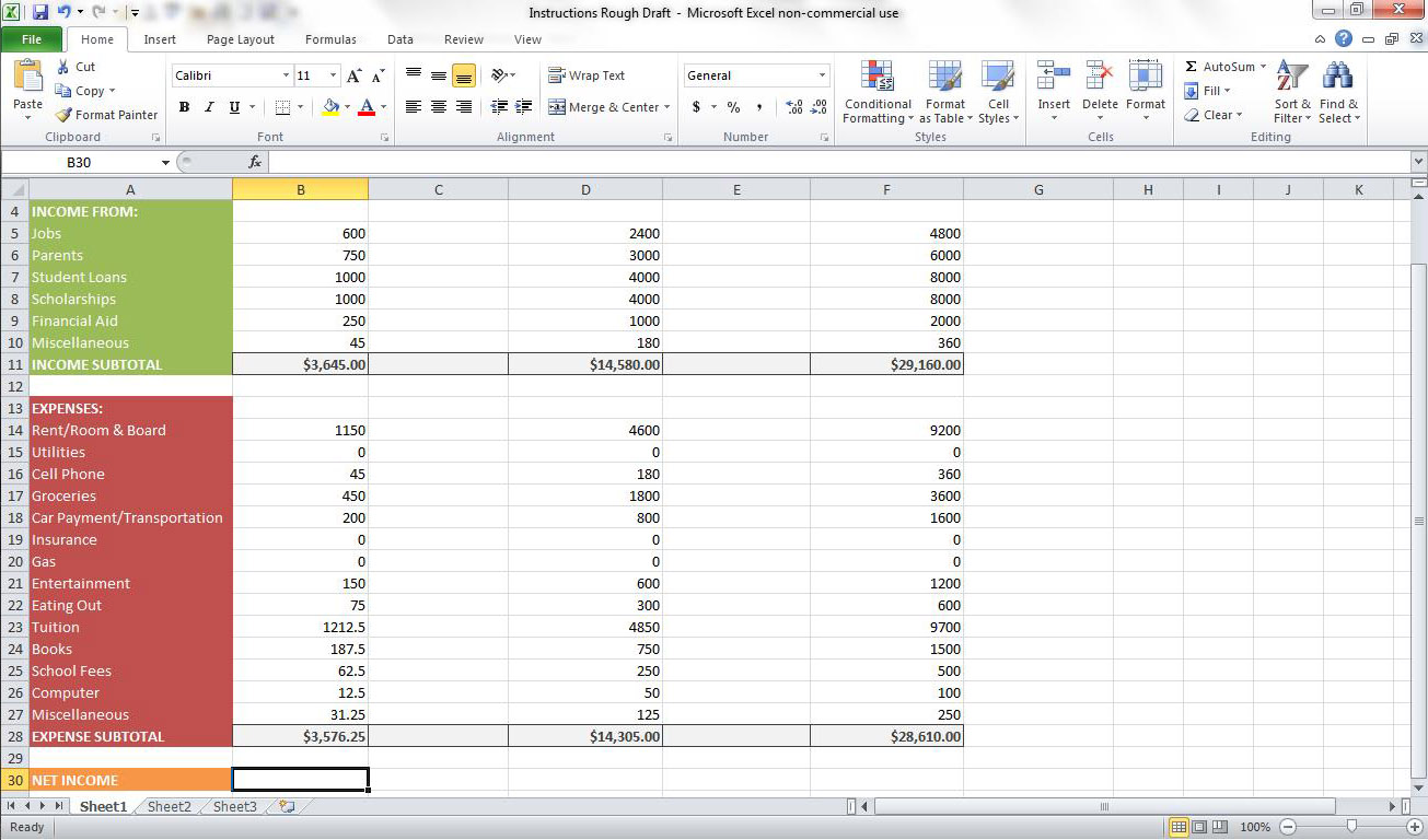
III. Now, select cells B11-F11 again and click on the drop-down arrow labeled “General” in the Number section of the toolbar. Select “Currency”.
IV. Once again, repeat the previous process for cells B28-F28.
II. Repeat this process for cells B28-F28 in the Expense Section.
III. Now, select cells B11-F11 again and click on the drop-down arrow labeled “General” in the Number section of the toolbar. Select “Currency”.
IV. Once again, repeat the previous process for cells B28-F28.
Determine and Format Net Income
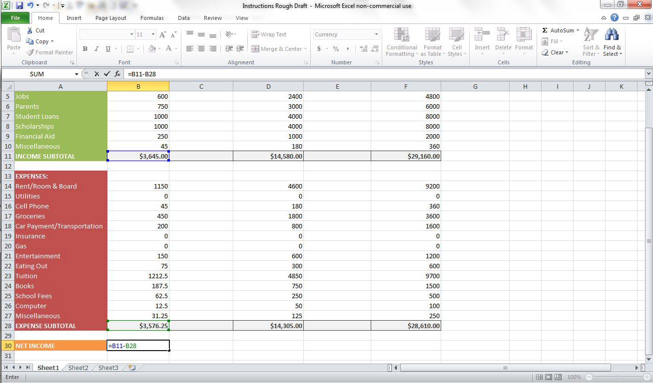
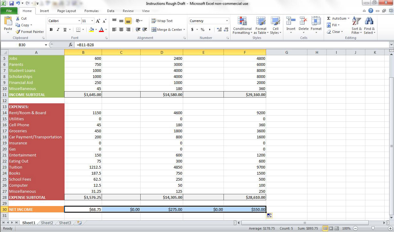
I. Select cell B30 and enter the formula “=B11-B28”. (Note: Net Income=Income-Expenses. This is illustrated by the formula used across row 30.)
II. Now, use the AutoFill feature to fill in the totals across Row 30 (From Column B through Column F).
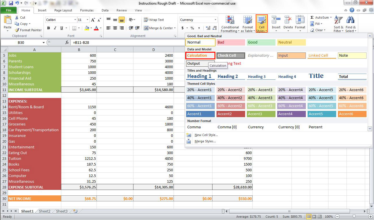
III. Format cells B30-F30 by selecting all of them and clicking “Cell Styles” located on the toolbar and then choosing “Calculation”.
II. Now, use the AutoFill feature to fill in the totals across Row 30 (From Column B through Column F).
III. Format cells B30-F30 by selecting all of them and clicking “Cell Styles” located on the toolbar and then choosing “Calculation”.
Analyze Budget
After completing the budget it is important to look over and analyze the different aspects of it. This involves looking at all the categories and looking for places where you might be able to cut back on spending and if possible increase income. While it is more difficult to increase income than it is to cut expenses it is still tough for most people to reduce the amount they spend, When looking at what you are spending money on, the key is to separate your needs from your wants. Once you separate identify these expense subcategories it allows you to focus on trimming down the amount you spend on wants. It is also wise to invest money into savings whenever possible, although, as most college students will attest to, this is easier said than done.