From MR Images to Electric Field: Modeling Transcranial Magnetic Stimulation

Introduction:

This set of instructions will show you how to use SimNIBS to turn MR images into a 3-dimensional model and then how to use the finite element solver SEMCAD X to illustrate the electric field induced from Transcranial Magnetic Stimulation (TMS). Why might someone want to do this? TMS is growing rapidly as a noninvasive tool for brain stimulation with applications treating chronic, drug-resistant depression, boosting memory, and in the world's first noninvasive brain-to-brain communication system. This technique uses a system of coils, and a large pulse of current to induce a varying magnetic field near the head of persons receiving TMS and this pulse induces an electric field in the brain that alters neural activity. Using finite element simulations, we can see the electric field that TMS creates in the brain and attempt to predict how the person receiving TMS will respond to treatment. Cool, right?

Prerequisites:

• SEMCAD X (Expensive)
• SimNIBS (Free)
• Set of T1 and T2 MR images each in a compressed NIfTI file (free set available on SimNIBS website)
• Basic knowledge of using Terminal in a linux environment
• Engineering or science background (nice but not necessary)

The scope of this instruction does not cover the installation of SEMCAD X and SimNIBS. If you already have SEMCAD X but not SimNIBS, follow the following link to see if you have a computer that will support SimNIBS and proceed through the listed steps. If you do not have SEMCAD X, you can email sales@beacon-tech.com to discuss purchasing the software suite, but you may be better suited to use SimNIBS for finite element simulations (not covered in instructions).

Expectations/Goals of Project:

This project may take a day or two to complete, depending on how precise you want the results to be. A user comfortable with this process should expect to spend less than an hour of their own time going through these different steps, but there will still be 12+ hours of time that the computer will take to segment the medical images and run necessary simulations where no user interaction will be necessary.

The project has two major goals, first to use MR images to create a head model, and second to use this model to illustrate the electric field induced in the brain via TMS. These two major goals are relatively independent of one another so you can choose to create head models without simulating TMS and you do not have to create a new head model every time you want to run a new simulation.

Once the simulations are complete, you will be able to view the resulting electric field.

To begin this step, you should be using your computer with SimNIBS installed and have 2 sets of MR images in a known folder. If this is complete, continue to the following procedure:

1. Open an instance of Terminal
2. Change the Terminal instance's directory to the folder containing your MR images
3. Enter the following command into Terminal: "mri2mesh --all modelName image1.nii.gz image2.nii.gz". ***
4. Wait for the computer to finish segmenting images and writing to 3D model (may take from 8-24 hours depending on the quality of the computer).

*** modelName indicates the final name of the model (enter whatever you wish for this field), and image1/image2 represent the two sets of images.

Do not continue to next step until process is completed.

Congratulations! You have officially made your first model. Now we are going to take this model and save it in a format that can be used with SEMCAD X. All of the files created from SimNIBS can now be found in the folder where you stored your MR images. The files we are particularly interested in have the extension ".stl", these include all the different model components created from the MR images.

1. Open folder containing original MR images and results.
2. The files seen in the image above will now be present.
3. Open a new instance of terminal.
4. Type the following command to open the model visualization tool GMSH: "gmsh&". This will result in a blank white window and corresponding toolbar opening.
5. Use the new toolbar to open the file "cerebellum.stl" by clicking File->Open and proceeding to the "cerebellum.stl" file in your working directory. The result should look somewhat similar to the image seen above, variation may be seen due to differences in MR images.
6. Save the file in binary formatting click File->Save As then clicking "Ok".
7. A new dialog will appear saying that a file with that name already exists, press "Replace" to proceed anyways.
8. A final dialog will appear, in the "format" field, change the selected option from "ASCII" to "Binary" and select "Ok" to reformat the model.
9. Next, all the other portions of the model will need to be reformatted. Select File->Open, and then proceed to open the file "CSF.stl" in the folder with your results. Follow the process described in bullets 6-8 for the "CSF.stl".
10. Continue by opening and saving "gm.stl", "skin.stl", "skull.stl", "wm.stl", and "ventricles.stl" using this same process.

You have now created a model and saved it in a format compatible with SEMCAD X.

At this point, you should have all components of your model saved as binary STL files. If SimNIBS is located on a separate machine from SEMCAD X, move the new STL files to the machine with SEMCAD X. Now, in this step you will import the new model pieces into SEMCAD X and create a simplified TMS coil.

1. Open SEMCAD X
2. Select File->Import Model->STL File.
3. In the resulting dialog window that appears, go to the folder containing your STL files (cerebellum, csf, gm, skin, skull, ventricles, and wm). Select all the files and press "OK" to import the files. If SEMCAD X fails to import any of the files and opens a new dialog with an error message, this means a mistake was made in the reformatting of the model from "ASCII" to "Binary"; to fix this error, go back to Step 2 and go reformat the failed model components using the same procedure previously described.
4. With all of the model components imported, the model should look similar to the first figure seen above and the part's list should contain all the same components.

With the model imported, we will now create a coil for TMS.

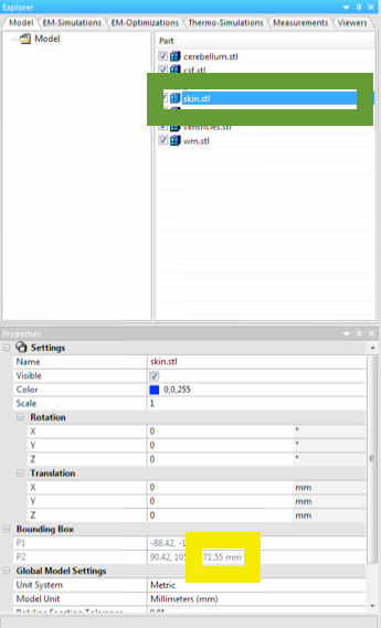
1. First we need to find where to place the coil. To do this, select "skin.stl" as seen in the green box in the second figure, and note the top of the head as the Z component of the bounding box P2 as seen in the yellow box. In this case, the demonstrated point is 71.55 mm so we will later place a coil at 76.55 mm, 5 mm above the top of the head. The 5 mm account for the outer covering of a TMS coil.
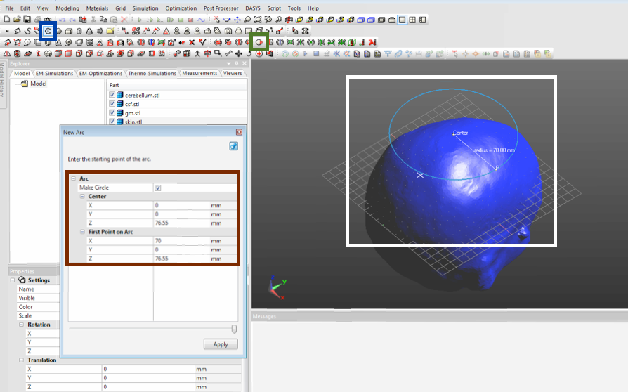
2. Now we will make an arc to represent a circle. Start by clicking the "arc" tool as seen in the blue box in the third figure.
3. Then a dialog will appear as seen in the maroon box in the third figure, in the two data-fields that represent data in the Z dimension, enter the desired height of the coil, in this case it will be 76.55 mm as described in the first bullet.
4. In the second box for the X dimension, enter 70 mm (this will be radius of circle).
5. Check that your dialog's entry fields have the same values as those in the maroon box (substituting 76.55 for your value for height), and if all fields match select "Apply" to make the coil.
6. Exit out of the dialog.
7. Confirm that the newly created coil looks like the blue ring in the white box of the third figure. If it does not, delete the circle named "Arc 1" under "Part" ("Arc 1" will be below the "wm.stl" object) by right clicking on the object and selecting "Delete". Then the previous bullets to recreate the circle.
8. Select "Arc 1" in the "Part" box and then click the "LF Current Source" button as seen in the green box in the third image to make the circle a low frequency current source.

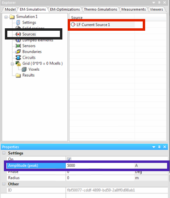
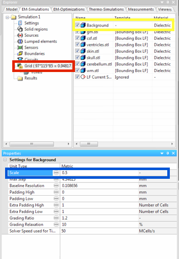
In this step you will set different parameters associated with the simulation, and begin running the simulation. After the simulation is initialized, the duration of the simulation will depend on the speed of the computer being used and a variation of different settings but could be as little as one minute or as long as one day.

Settings (first image):

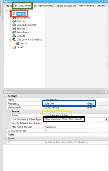
1. In this step, follow the first picture seen above. Start by selecting the "EM-Simulations" tab as seen in the green box, then click on the "Settings" label seen in the red box.
2. Follow by making sure the values in the blue, yellow, and black box are "2.5e-6", "Low Frequency Solver", and "Magneto Quasi Static (Biot-Savart)" respectively.

Solid Regions (second image):

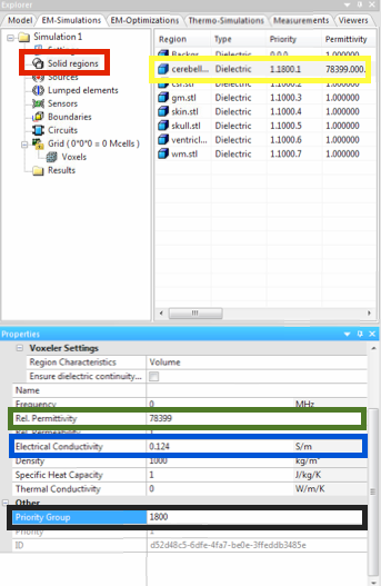
1. Next you will change the electrical properties of each material. Start by selecting "Solid Regions" as seen in the red box.
2. Then click on the "cerebellum.stl" file as seen in the yellow box.
3. Change the permittivity, conductivity and, priority group of the object to 78399, .124, and 1800, as seen in the green, blue, and black box.
4. Next we will change the attributes of the remaining materials by following the same process as described in bullets 2-3 only using different values.
5. Select "gm.stl" and change permittivity, conductivity, and priority group to 78104, .104, and 1800 respectively.
6. Select "wm.stl" and change permittivity, conductivity, and priority group to 34282, .065, and 1900 respectively.
7. Select "skin.stl" and change permittivity, conductivity, and priority group to 1135, 0, and 500 respectively.
8. Select "skull.stl" and change the permittivity, conductivity, and priority group to 1435, .02, and 600 respectively.
9. Select "ventricles.stl" and change the permittivity, conductivity, and priority group to 102, 2, and 2000 respectively.
10. Select "csf.stl" and change the permittivity, conductivity, and priority group to 102, 2, and 700 respectively.

Sources (third image):

1. Now we will adjust the parameter for our models coil. Select the "Sources" tab as seen in the black box.
2. Select "LF Current Source 1" as seen in the red box.
3. Change amplitude to 5000 amps as seen in the purple box.

Grid (fourth image):

1. Select "Grid" as seen in the red box.
2. A dialog will appear, press "Ok" to continue.
3. Select "Background" as seen in the yellow box.
4. Change the data entry under "Scale" to .5 as seen in the blue box. The smaller the scale, the more accurate the final results will be, but more accurate also means more computer time and larger files.

Voxels

1. Right click on the "Voxels" tab which is immediately below the "Grid" tab and select "Make Voxels".
2. Upon making voxels you will get a prompt telling you to save the file. Follow by saving the file in an appropriate location.

Results

• Right click on the "Results" tab which is immediately below the "Voxels" tab and select "Run".

Depending on the speed of your computer, the simulation should take approximately one minute. Longer simulations with more precise grids and more complicated coil designs can take several hours.

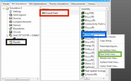
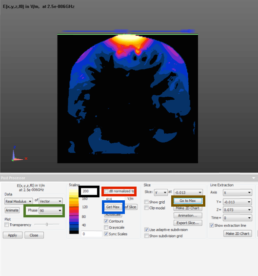
In this final set of steps, you will learn how to view the results of your simulation.

1. Start by going to "Results" and then clicking on "Overall Field" as seen in the first image.
2. Follow by right clicking "E(x,y,z,f())" and selecting "slice field view" as seen in the blue and green box of the same image.
3. This will bring up a dialog, click "Next".
4. Click "Next" again on the following dialog.
5. Change the phase to 90 degrees as seen in the green box of the second image.
6. Press the "Get Max" button seen in the blue box of the second image.
7. Press the "Go To Max" button seen in the brown box of the second image.
8. Uncheck the "dB normalized to" field as seen in the red box of the second image.
9. Enter "200" as seen in the data entry field in the black box of the second image.

Now you can see the electric field! The bright yellow portions represent portions of the head model with over 200 V/m and the black regions represent portions of the field with 0 V/m. If you are interested in learning more about what you can do with SEMCAD X or how you can visualize your data, play around with the different modeling tools in the toolbar or see the SEMCAD X Manual.