Creating a College Budget in Microsoft Excel

College students have many expenses to keep track of each month. It can be difficult to see the big picture of where the money is going as each month progresses. By creating a budget spreadsheet in Excel, college students can clearly see what expenses they have each month. By using the Google Drive app in their phones, they are able to see how much they can spend when they are out.

Collect data of your monthly income and expenses.

• Complete the instructions with the provided data set first.
• Once you have completed all of the instructions, and have your final pie chart, you may go back and create a new pie chart to input your own data that fits with your budget.

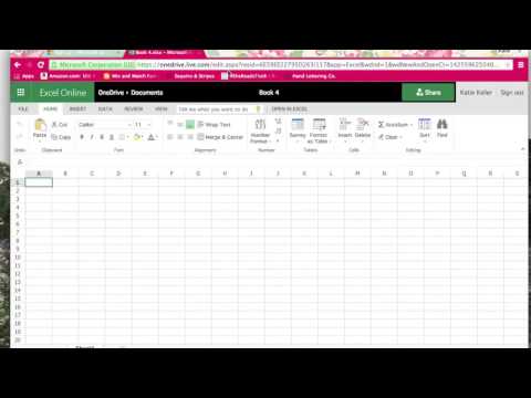
Open Microsoft Excel on your computer. If you don’t have Microsoft Excel, you can use Microsoft Excel Online.

• If you need to use Microsoft Excel Online, see the video.

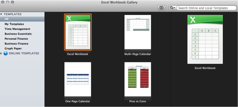
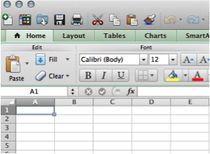
1. When you open Excel (either on your computer or using Excel Online), select the “Excel Workbook” in the Excel Workbook Gallery, which is located in the top left corner.
   
   • Do not use the Household Budget template. It is useful in budgeting for a household, but college students need a different kind of budget.
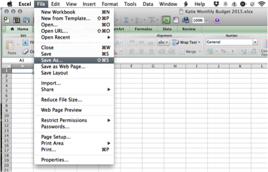
2. At this point, you want to save your work.
   
   • Click File > Save As at the top of your screen and save the spreadsheet as “[Insert Your Name] Monthly Budget 2015.”
   • Save it to the Documents folder on your computer.
3. Get familiar with how to move around the spreadsheet.
   
   • On the spreadsheet, go to column “A.” This is where the categories for data will be entered.
   • Under Column “A,” looking at the vertical list of numbers to the left, enter the first category across from number 1.
   • After you finish entering the first category, hit RETURN/ENTER to enter the next category.
   • Using the TAB key will help you move across columns--from column A into column B, for example.

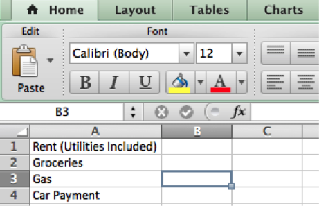
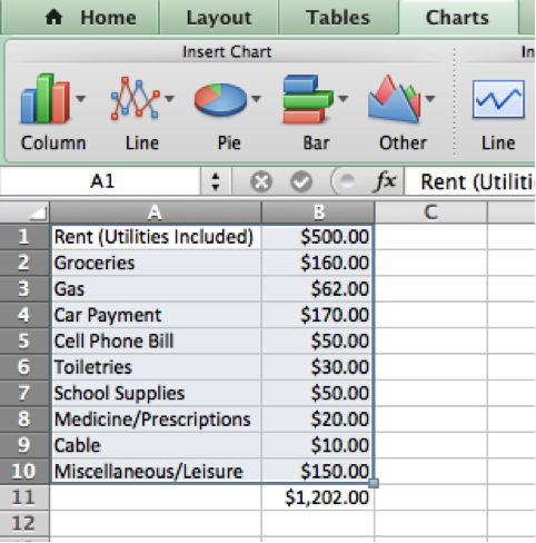
1. Type the following categories shown below in column A, in rows 1-10:

A1. Rent (utilities included)

A2. Groceries

A3. Gas

A4. Car Payment

A5. Cell Phone Bill

A6. Toiletries

A7. School Supplies

A8. Medicine/Prescriptions

A9. Cable

A10. Miscellaneous/Leisure

2. After you have entered all of the categories, you will need to expand the size of column A to the right to fit all of the words.

• When your mouse is on the spreadsheet in Excel, it should be shaped like a plus sign. To expand the size of column A, hover your mouse over the line between column A and column B in the shaded portion at the top. The mouse will turn black, with arrows pointing left and right. Double click with the mouse between column A and B until each category’s title fits in column A. You can also click and drag the mouse to the right or left to adjust the size of the column.
• As you enter the categories, the text will appear in the cell itself, but also in the ribbon at the top of the page. After you have officially inputted the category by hitting RETURN/ENTER, these categories can be edited or changed by clicking on the cell and editing in the ribbon on top of the spreadsheet.
• As you enter categories, be sure to continuously save your work. You can use File > Save, or Ctrl/Command + S to save.

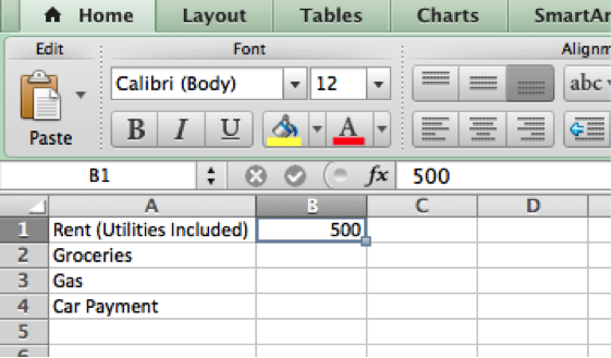
B1. 500

B2. 160

B3. 62

B4. 170

B5. 50

B6. 30

B7. 50

B8. 20

B9. 10

B10. 150

• On the spreadsheet, go to column B. This is where the values for the data will be entered.
• Under column B, looking at the vertical list of numbers to the left, enter the first value across from number 1.
• After you finish entering the first value, hit RETURN/ENTER to enter the next value.

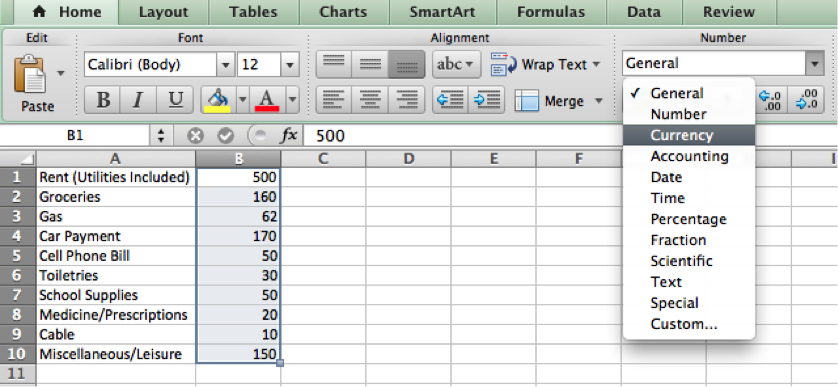
To make these quantities into currency, highlight the information in column B, and under the Home tab, find the drop down menu under Number and select Currency, instead of General. All of the quantities should now be in dollar amounts.

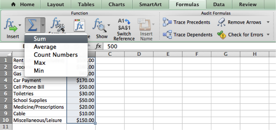
Now, highlight column B again, and click on the Formulas tab. Under the Formulas tab, click AutoSum.

• You can also click on the arrow next to AutoSum, which reveals a drop-down menu. Click Sum.
• All of the various expenses in the budget should all be added up, and the total will appear below the last data cell.

If you used our data, the total should be $1202.00

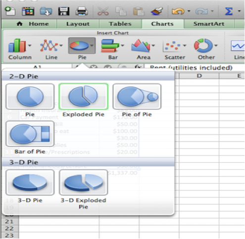
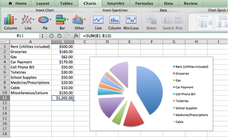
1. After entering data into column A and column B take the mouse to the upper left corner and click on cell A1 while holding the mouse down drag across column A and B down to number 10 to highlight.
   
   • Both of these columns should now be highlighted in blue.
   • Do not include the total sum in cell B11.
2. After the columns have been highlighted go up to main bar and click on Charts.
   
   • Another bar will appear that has the options of which cart you would like to use.
3. Click on Pie.
   • A drop down screen will appear with options of different pie charts to select.
   • Click on Exploded Pie.
4. A pie chart will appear on the Excel spreadsheet you are working on with the information obtained from the two columns.
5. To make the pie chart bigger go to any corner of the chart and hover the mouse over it, a two headed arrow will appear, then click in the lower right corner and drag the mouse out to resize the chart.

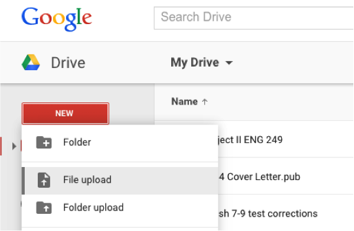
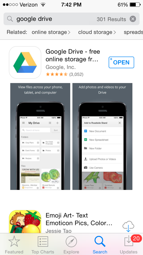
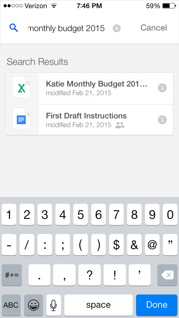
1. To use your newly created Excel spreadsheet on the go, you can upload the spreadsheet to Google Drive to use anywhere you have access to the internet. If you have a smartphone, you can use the Google Drive App to view your budget on the go.
   
   • The screenshots show the process on an iPhone, but it works the same on an Android.
2. To use Google Drive, you need a free Google account. If you don’t already have a Google account, you can go to this website to set up a free account: www.google.com/drive
   • If you already have an account, go to step 2.
3. Go to www.google.com/drive and sign in.
   • The Google Drive homepage will appear, including any documents you have created on Google Drive in the past.
4. Click on the orange box in the left corner that says NEW.
   • A drop down menu will appear. Select File Upload.
5. Select your budget from where you saved it and click Open.
   
   • A skinny box will appear in the lower right hand corner, which shows the uploading progress.
   • Once your spreadsheet is uploaded, it will appear as an Excel file in your Google Drive.
6. Now you need to download the free Google Drive app.
   
   • Go to the App Store and search Google Drive.
   • Download the app to your phone.
7. Open the Google Drive app on your phone and sign in using your free Google account.
   • Any documents you have on Google Drive are now available to view on your phone.
8. In the search bar at the top of the screen, type in the name of your spreadsheet: [Insert Your Name] Monthly Budget 2015.
   • Tap on the spreadsheet. You can now view your spreadsheet when you are on the go, so you know how much you can spend on groceries, coffee with friends, or while out shopping.