Constructing and Analyzing an Electric Guitar Pickup

The main goal for our project was to create a circuit that accurately modeled/resembled the characteristics of a guitar pickup. Since we did not have access to the physical pickup until later in the project, we started by making our circuit design and hardware based on bode plots for a Fender Stratocaster Bridge (no integrator), a low pass filter. However, once we got access to and measured our actual pickup, a Musiclily 50MM Single Coil Squier pickup, we observed that the pickup behaved as a high pass filter and varied significantly from our original circuit. Therefore, we redesigned our RLC circuit by changing component values and adding a voltage divider to introduce a negative gain term in the bode plot. The resulting frequency response function of the RLC circuit matched closely measured response of the Squier guitar pickup.

• 2 x 1 kOhm Resistor
• 1 x Musiclily 50MM Single Coil Squier pickup
• 1 x 10 kOhm Resistor
• 1 x 47 kOhm Resistor
• 1 x 470 kOhm Resistor
• 1 x 4.7 nF Capacitor
• 1 x 50 mH Inductor
• 1 x Oscilloscope 
• 1 x BNC cable
• 2 x Oscilloscope Probes

Once the guitar pickup arrived, we measured its frequency response with the oscilloscope. To achieve this, we attached the output of the Frequency Generator (which generated a 5 Vpp sine wave with varying frequencies) directly to a 50 mH toroidal inductor. The inductor generates an oscillating magnetic field that can be sensed by the pickup, when it is held directly on top of the cylindrical magnets of the pickup. The setup is shown below:

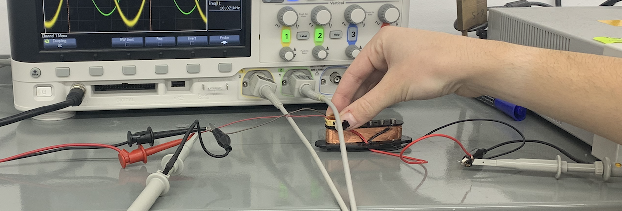
Figure 5: The measurement setup for the Squier Pickup. The input voltage was connected to a toroidal inductor fastened to the pickup’s magnets in order to create a magnetic field for the pickup to read. The output voltage was connected to the two wire terminals located at the bottom of the pickup.

By varying the frequencies from 3 kHz to 100 kHz, we obtained different values for the Vout of our Squier pickup. Below is a screenshot of the oscilloscope measurement setup for the Squier pickup at a couple of the chosen frequencies. 

Figure 6: The oscilloscope measurement setup used in our results for the Squier Pickup. The green signal is the input voltage and the yellow is the output voltage. 

Once we had the voltages in and out for the Squier pickup, we calculated the log magnitude using the same Equation 1 as before and plotted the values over the frequency to get our bode plots. The bode plot is shown below.

Figure 7: The Bode plot for our hardware circuit 

The Squier pickup behaves as a high-pass filter, with a resonant peak, shown in Figure 7. The resonant peak magnitude is approximately -25.680 dB with a steady state magnitude of -35.494 dB. Unfortunately, this does not match our hardware circuit from section 3, which was a low-pass filter. Additionally, the values of our magnitudes and corner frequencies did not line up. The corner frequencies were about a decade apart from each other, with the circuit having a corner frequency of 110 kHz and the Squier pickup 10 kHZ. The output of our circuit produced values in the 1-7 V range while the Squier pickup in the mV range. 

There are a couple of reasons why our circuit model did not line up with the Squier pickup. The main concern is that pickup itself is not the same model or manufacturer as the one we designed in hardware. As mentioned previously, the values chosen were modeled after measurements for a Stratocaster pickup we found. The Squier pickup that we were able to purchase for the project did not have component values readily available. Because of this, we had to estimate the behavior and values based off of other pickups when creating our circuit, and did not know that the results of the actual pickup would behave this way. 

Something else that we noticed in this phase is the major difference in corner frequency and why our initial design did not make sense for our intended purpose. Typically, human ears can only hear up to 20 kHz, so a 10kHz corner frequency makes much more sense than 100kHz.

Once we had the measured corner frequency and behavior of the pickup from section 4, we began designing a revised version of our RLC circuit. We discovered that the largest inductor we could implement was 50 mH so we used that and the resonant frequency of 10 kHz to solve for our capacitor and resistor values. Once we had those values, we simulated the circuit using software and observed the corresponding bode plot. This created a signal of the correct behavior, but the gain was a bit lower than what we wanted. To fix this, we used a voltage divider before the RLC section of our circuit, using values from the steady state voltages (the values to the right of the resonant peak in Figure 7). The calculations are shown below in the references and appendix section at the bottom of this document.

The final circuit design is shown below in Figure 8. Using software to find the simulated bode plot, we found that our circuit portrayed the expected behavior. 

Figure 8: Our Final Circuit Schematic

To build and test our circuit in hardware, we used the following components. A more detailed list is located in the references and appendix section at the end of this document.

• 2x 1 kOhm Resistor
• 10 kOhm Resistor
• 47 kOhm Resistor
• 470 kOhm Resistor
• 4.7 nF Capacitor
• 50 mH Inductor
• Oscilloscope 
• BNC cable
• Oscilloscope Probe 

Using a breadboard, we constructed the circuit shown below in Figure 9. We then connected the input voltage wires and ground to a BNC cable connected to the Wave Generator function on the oscilloscope set to a sinusoid with an amplitude of 5 Volts. The output wire was connected the the oscilloscope probe.

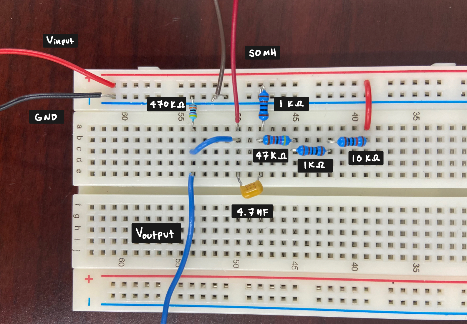
Figure 9: The breadboard layout for our final circuit

Taking the output voltage at varying frequencies, we recorded the results of our circuit. We again used Equation 1 to calculate the log magnitude of the values for the bode plot. Plotting the magnitude over the frequency, we received the bode plot shown below in Figure 10. The resonant peak (at 10 kHz) is approximately -26.702 dB and the magnitude during steady state (at higher frequencies) is -34.399 dB.

Figure 10: The bode plot for our final circuit

Overall, the behavior of our final circuit is consistent with the Squier pickup and the frequency response functions match extremely well. Comparing Figure 7 to Figure 10, we see that the resonant frequency for both devices is 10 kHz. The peak magnitude for the RLC circuit is -26.702 dB, while the magnitude for the Squier pickup is -25.680 dB (a difference in magnitude of approximately 1 dB). In addition, the steady state voltage values at high frequencies for the RLC circuit was -34.399 dB, while the value for the Squier pickup was -35.494 dB. These values are within 5% of the calculated values for the Squier pickup and are therefore pretty close. It is also important to note that this difference can be accounted for by manufacturing imperfections in circuit components (ex: resistors having slightly different resistances).

In conclusion, a hardware circuit can be used to perform as an electrical guitar pickup, taking in sinusoidal voltages at varying frequencies and using a high pass filter with resonance to amplify certain frequencies such as guitar string oscillations and nullify others. Through this project we learned a lot about the underlying theory behind circuit components such as inductors. We also learned how pickups exploit the unique properties of magnetic fields to generate sound in a controlled manner. This project dives into the intersection of physics and engineering, providing insights into the practical applications of electromagnetic principles such as Faraday’s law.

Finally, we also gained some practice designing a circuit from a desired frequency response. In this sense, we honed our ability to translate conceptual concepts covered in class into practical implementations.