Cellular Automata and an Implementation of Conway's Game of Life

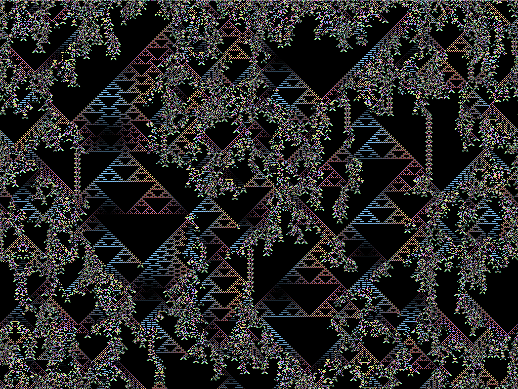
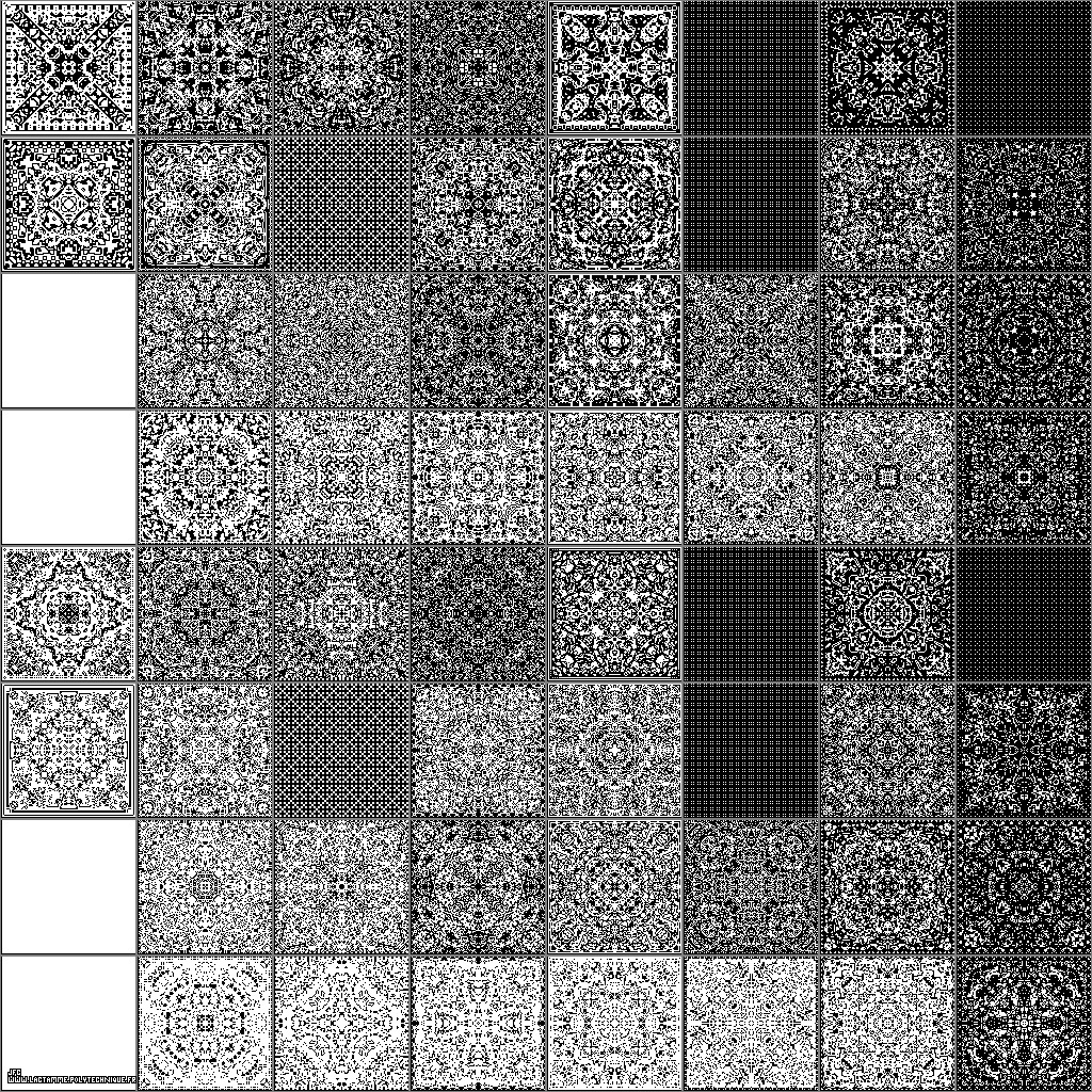
As far as I know, there have only been two instructables articles on cellular automata which can be found here and here. Neither article explains what cellular automata are, why they are interesting, or how one can implement them in code. So, I decided to write my own instructable so that others may develop an interest and may begin their own coding experiments. Since Conway's Game of Life is the most common cellular automata I will focus on it for the majority of the article. By the end, I will have covered the following

• a general description and definition of cellular automata
• cellular automaton applications
• overview of Conway's Game of Life
• how to implement Life as a program in C++
• an explanation for this program and its use

I have attached some photos of 2D cellular automaton systems.

Basically cellular automata are discrete systems that are really interesting to study. They have a range of applications and help explain fundamental concepts in computing and discrete mathematics. Most cellular automata consist of a collection of cells (typically projected onto a grid) that change over time according to some set of rules. Cellular automaton systems are characterized by a certain cellular space and a transition function. A cellular space is described as a regular lattice in a specified number of dimensions (a lattice is like an organized collection of cells, in 2 dimensions it would be a flat grid).

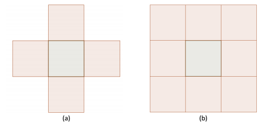
Each cell has a specified number of states. A neighborhood includes the state of cells adjacent to a particular cell and is often used by the transition function in determining future states. In two dimensions, there are two main types of neighborhoods: the Moore neighborhood and the von Neumann neighborhood. The Moore neighborhood includes the eight cells surrounding one cell while the von Neumann neighborhood excludes the four corner cells in the Moore neighborhood. The difference between the two is depicted in the picture where (a) gives the general von Neumann neighborhood and (b) gives the general Moore neighborhood.

Well, besides being fascinating cellular automata do have practical applications. For example, cellular automata are useful in modeling fluid dynamics and creating parallel processing units. They can also be employed in cryptography systems. Moreover, they can model traffic flow and provide key insight in extant problems of pure mathematics. So, in short, a lot of people care about cellular automata and they are used in a multitude of ways.

The Game of Life is a specific type of cellular automata. It was developed by John Conway in the 1970s who hoped to study population patterns. Essentially, it is a 2-state 2D automata with a moore neighborhood. By convention, cells are dubbed "alive" or "dead" based on their state. The rules are simple and can be summarized as follows

• A live cell dies from loneliness if it has zero or one live bordering members
• A live cell remains alive if two or three members are alive in its neighborhood
• With more than three live members, a live cell dies from overpopulation
• If a dead cell's neighborhood includes exactly three live members, this cell is "born" and becomes alive

The collection of these rules compose the transition function which takes as input a particular cell's state and the states of the cells in its neighborhood, then outputs the state of that cell in the next generation. Give a cellular automaton that includes a collection of live and dead members, the transition function would be applied to every cell in order to determine the configuration of the automaton in the next generation.

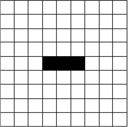
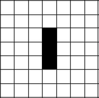
Perhaps a simple example can help describe how this transition function is applied to determine the evolution of a cellular automaton. Consider three live cells in a row, each adjacent to another, surrounded by dead cells in a grid. This configuration is denoted in one of the pictures. By convention, the live cells are colored black, and in this case, they form a horizontal bar across the grid. To determine how this configuration changes in the next generation, we apply the transition rule to each cell of interest. Suppose we start with the center black cell. It has two live neighbors (one to the right and one to the left). Thus, according to the rules previously outlined, it remains alive. Notice that the other two black cells each have one live cell in their respective neighborhoods. So, they each die in the next generation. There are also a number of white cells to consider. Naturally, most of the dead cells will remain dead because they have zero live cells, but a few will come to life. Namely, the cells directly above and below the center black cell will become alive because they each have three live neighbors in their respective neighborhoods. Hence, when all of these changes are applied to the system, the resulting configuration would resemble the second picture posted which depicts the live cells as a vertical bar.

When this configuration is rotated 180° it returns to the original configuration (i.e. a horizontal bar). It follows that this configuration will simply oscillate from horizontal to vertical bar each generation. In fact, it is a well known configuration and is commonly referred to as a "blinker."

When Conway originally invented the Game of Life, he implemented the simulation on a computer so that he could practically view the evolution of the system. By encoding the rules into a program, we can easily manipulate the start configuration and view subsequent behavior. Such experimentation is often essential to the aforementioned applications and can be sued for all sorts of research endeavors. I have created an assortment of simulation programs for my own research; some of which can be found here. For this instructable, I will be covering the basic outline of an implementation in C++. I have divided the task into several essential functions.

• Create automaton
  • Create the initial configuration
  • store this configuration
• Update automaton
  • apply transition rule to each cell of interest
• Check automaton
  • ensure that the live cells are still within containment boundaries
• Output current configuration
  • allows one to view evolution of automaton
  • outputs to console
• Write current configuration
  • output information to text file if needed

This step regards the creation of the initial configuration. If you're using C++11, I think the easiest way to store the automaton involves vectors. This way, the size of the automaton is adaptable. Since the stored data maintains a 2-dimensional form, it is best to store the automaton as a 2-dimensional vector (i.e. vectors within a vector). With this setup, the automaton is viewed as a grid. Each row of the grid is stored as a vector. Each row vector is in turn stored in the main vector. Suppose we want to start out with a 10 cell by 10 cell grid. The vector declaration would resemble the following:

vector< vector > grid(10, vector(10, 0));

This declaration not only creates a 10x10 grid but also initiates each cell value to 0 (or dead). Now you can implement whatever code to change to the values of the cells initially alive. For example, suppose I want the cells initially alive to form a solid square on the grid (from their coloration differences as noted before), then I would implement a loop resembling the following:

for(int i=2; i<8; i++)
{

for(int k=2; k<8; k++)

grid[i][k]=1;

}

This creates the desired vector termed grid, which I can subsequently use to store the cellular automaton. Notice that I have left the two outer layers of cells in a dead state. These layers are essential to the automaton. I will explain them in Step 7. As a separate function called newAutomaton() this segment of the program would resemble the following:

vector< vector > newAutomaton()
{

vector< vector > grid(10, vector(10, 0));

for(int i=2; i<8; i++)
{
for(int k=2; k<8; k++)

grid[i][k]=1;

}

return grid;

}

This segment can easily be adapted to fulfill the requirements of the task, but it serves as the basis for the creation component of the simulation.

This step applies the transition rule to each cell of interests. Before addressing this construction, it is important to address the two layers of dead cells around the main configuration. These cells allow the automaton to expand if necessary. Normally, a cellular automaton in Conway's Game of Life evolves on an infinite grid; however, it is more practical to represent this grid in a finite virtual container (e.g. a vector). This change necessitates a "buffer layer" of dead cells to allow for the expansion of the automaton. So, we should check all of the cells in the grid including the innermost buffer layer (remember, the outermost buffer layer would consist of cells whose neighborhoods have zero live cells, so they remain dead and do not need to be considered). The header of the function would resemble the following (I have named the function updateVec).

vector < vector > updateVec(vector< vector > grid)

Essentially the function works by creating a new 2-dimensional vector and filling the cells with the correct values of the updated cells from the original grid. The entire code segment would resemble the following.

vector< vector > updateVec(vector< vector > grid)

{

int size=grid.size();

vector< vector > newgrid(size, vector(size));

int c1=1;

int c2=1;

while(c1

{

while(c2

{

int sum_neighborhood=grid[c1+1][c2]+grid[c1][c2+1]+grid[c1+1][c2+1]+grid[c1-1][c2-1];

sum_neighborhood+=grid[c1-1][c2]+grid[c1][c2-1]+grid[c1+1][c2-1]+grid[c1-1][c2+1];

if(grid[c1][c2]==0&&sum_neighborhood==3)

newgrid[c1][c2]=1;

else if(grid[c1][c2]==0&&sum_neighborhood!=3)

newgrid[c1][c2]=0;

else if(grid[c1][c2]==1&&(sum_neighborhood==2||sum_neighborhood==3))

newgrid[c1][c2]=1;

else if(grid[c1][c2]==1&&(sum_neighborhood!=2&&sum_neighborhood!=3))

newgrid[c1][c2]=0;

c2++;

}

c2=1;

c1++;

}

return newgrid;

}

Note that the initialization of sum_neighborhood took place over two lines due to spatial constraints. The iteration began at 1 and ended before size-2 in order to avoid wasting time checking the outermost buffer layer.

This step ensures that two buffer layers remain surrounding the central automaton. The check function should run after every update. It works by checking the outer two layers for live cells. If it finds at least one, it runs a subroutine to expand the automaton by a layer of dead cells. The code for this function titled checkVec() would resemble the following.

vector< vector > checkVec(vector< vector > grid)

{

int size=grid.size();

int sumElementsOuter=0;

for(vector::iterator j=grid[0].begin();j!=grid[0].end();j++)

sumElementsOuter += *j;

for(vector::iterator k=grid[size-1].begin();k!=grid[size-1].end();k++)

sumElementsOuter += *k;

for(int m=1; m

sumElementsOuter=grid[m][0]+grid[m][size-1]+sumElementsOuter;

//add up the sum of the states in the layer right before the outer

int sumElementsIn=0;

for(vector::iterator x=grid[1].begin();x!=grid[1].end();++x)

sumElementsIn += *x;

for(vector::iterator y=grid[size-2].begin();y!=grid[size-2].end();++y)

sumElementsIn += *y;

for(int m=2; m

sumElementsIn=grid[m][1]+grid[m][size-2]+sumElementsIn;

if(sumElementsOuter>0)

{

//gird needs to be updated to have two new outer layers

grid.insert(grid.begin(), vector (size, 0));

grid.insert(grid.begin(), vector (size, 0));

grid.push_back(vector (size, 0));

grid.push_back(vector (size, 0));

int rows2=0;

int col2=0;

while(rows2

{

grid[rows2].insert(grid[rows2].begin(), 0);

grid[rows2].insert(grid[rows2].begin(), 0);

grid[rows2].push_back(0);

grid[rows2].push_back(0);

rows2++;

}

}

else if(sumElementsIn>0)

{

//gird needs to be updated to have one new outer layers

grid.insert(grid.begin(), vector (size, 0));

grid.push_back(vector (size, 0));

int rows2=0;

while(rows2

{

grid[rows2].insert(grid[rows2].begin(), 0);

grid[rows2].push_back(0);

rows2++;

}

}

return grid;

}

Sorry if the formatting is off. All of these functions can be found here where the code should be easier to read. Also, note that some of the functions rely on iterators. So, be sure to include the iterator library in the include directive at the beginning of the program.

This function is optional and simply outputs the current configuration to the console. I have termed the function outVec(). This function resembles the following.

void outVec(vector< vector<int> > grid)

{

int size=grid.size();

int counter1=0;

int counter2=0;

while(counter1<size)

{

while(counter2<size)

{

cout<<grid[counter1][counter2];

if(counter2+1==size)

cout<<endl;

counter2++;

}

counter2=0;

counter1++;

}

cout<<endl<<endl;

}

In this case, the program outputs a 1 if the cell is alive and a 0 if the cell is dead. A simple conditional statement can change the representations of the cell states to any character (for example, whitespace for a dead cell and * for live cells or something along those lines).

Sometimes it may be useful to write the automaton configuration to a text file. The function to complete this action is analogous to the outVec() function. If the function is called out2file() it would resemble the following

void out2file()

{

ofstream generations("generations.txt", ios_base::out | ios_base::app);

int size=grid.size();

int counter1=0;

int counter2=0;

while(counter1<size)

{

while(counter2<size)

{

generations<<grid[counter1][counter2];

if(counter2+1==size)

generations<<endl;

counter2++;

}

counter2=0;

counter1++;

}

generations<<endl<<endl;

generations.cloese();

}

Note that in order to use this function, I would have already created a text file called generations. Also, every execution of this function appends the file so that the configurations would accumulate. If you want to reset the contents of the file every time it is opened simply replace ios_base::app with ios_base::trunc. Again if desired, the symbols associated with cell states can be altered to any character with a simple conditional.

With these functions, you can begin to construct a multitude of programs that involve simulating cellular automata in Conway's Game of Life. Again, most of these functions can be found at https://github.com/cakoch10/Patterns_in_Game_of_L... Of course, to run these functions one would need to construct a simple main() function. In the main function, it would be useful to construct the initial grid vector, then create a loop that runs the update function and checks the automaton. Ultimately though, the next step of this instructable is left for the reader to decide. Only one's imagination can limit the kinds of projects that follow from this simple implementation.

Thanks for reading.