Audio App With a Built-in Equalizer

by AlePalma in Circuits > Audio

36 Views, 0 Favorites, 0 Comments

Audio App With a Built-in Equalizer

Eq_Eq_on.JPG
Eq_Eq_on_2.JPG

I will show you how I made an audio app in MATLAB with different functionalities like an equalizer or a real time spectrum analyzer. I will go step by step explaining how I programmed all the parts and the problems I faced during the whole process.

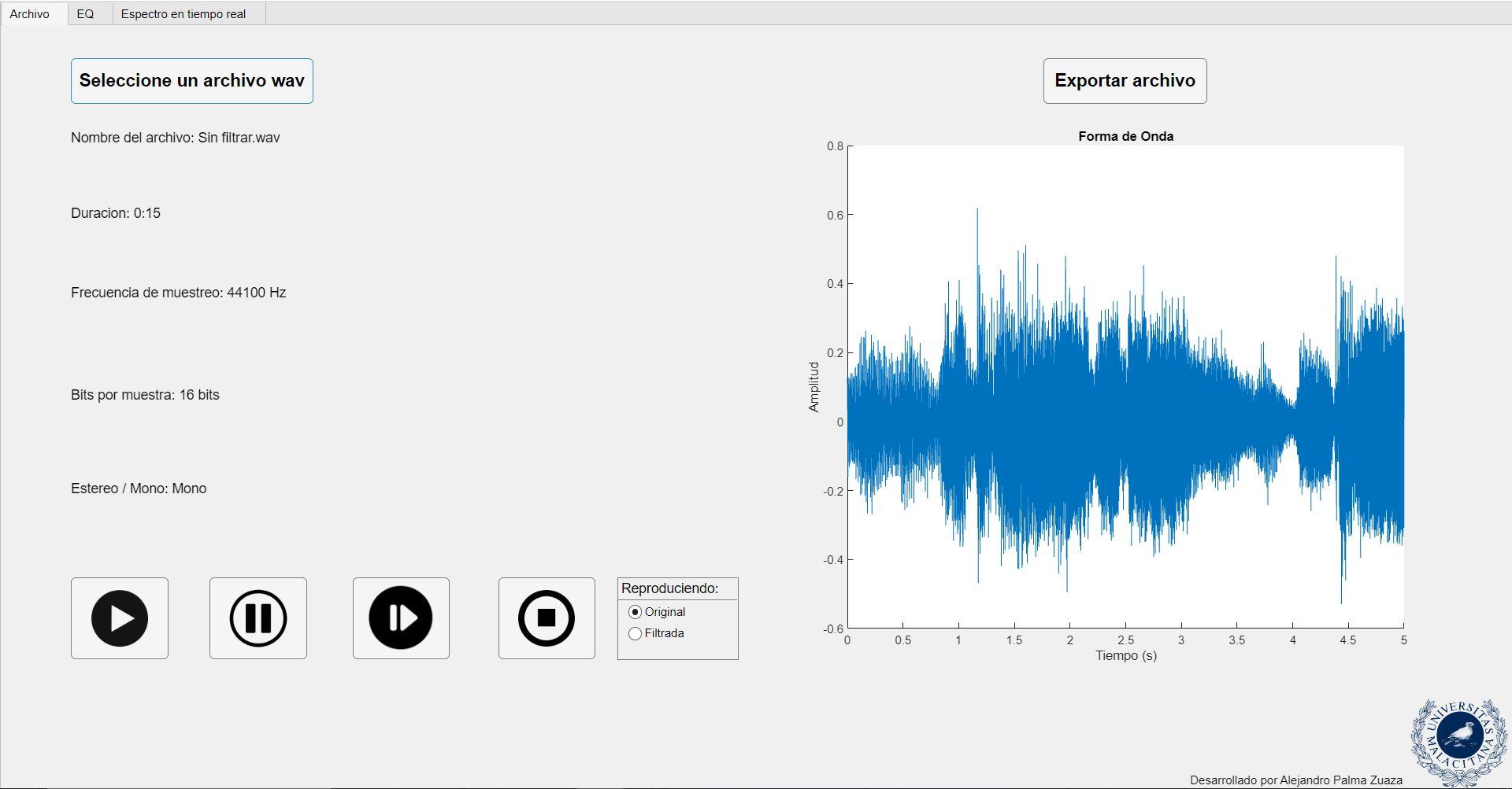
The app has 3 main pages: Archivo, Eq and Espectro en tiempo real. We will go trough each one but starting with Archivo, which is the first thing you see once you open the app.  

Supplies

  1. MATLAB

Downloads

Archivo

Eq_Archivo.JPG

As I said, the Archivo page is the first thing you see. To start with, you need to choose an audio file from your storage. In order to do that, you need to press the Seleccione un archivo wav button. I posted the whole code in the supplies, but with each part i will put the piece of code used. The comments of the code are in spanish.


  1. Seleccione un archivo wav button. It will open a dialog box to choose the .wav file. Code used:
app.archivo = uigetfile('.wav', 'Seleccione un archivo .wav');
info = audioinfo(app.archivo);
[app.signal_entrada, app.fs] = audioread(app.archivo);
app.NombredelarchivoLabel.Text = ['Nombre del archivo: ', app.archivo];

First you select the file, save it in app.archivo and save all the information in info. This will be used later to display some information about the file like the duration, the frequency rate or the bit depth.


  1. Play, Pause, Resume and Stop button. These ones are used to handle the playback of the file.

In Matlab there is a function which creates and audio player based on an audio file. This file is app.signal_entrada which we saved before. We create the audioplayer with this command:

app.reproductor = audioplayer(app.signal_a_reproducir, app.fs);

And once this is done we use stop(app.reproductor) to, for example, stop the playback.


  1. Reproduciendo Box. In this one, you can choose to play the original file or the filtered one. Depending of the one you choose, it will reset the audio player with the desired file.


  1. Exportar archivo button. It is used to export the filtered file to anywhere you want in your PC.
[filename, filepath] = uiputfile('*.wav', 'Guardar archivo de audio como');
FullFileName = fullfile(filepath, filename);
audiowrite(FullFileName, app.signal_filtrada, app.fs);

With this piece of code, you pick the folder of destination and then you write the file on the path with the matlab function audiowrite.


  1. Soundwave.

On the right side there is a graph which shows the soundwave of the audio file. It shows the first 5 seconds of the audio and is updated every 5 seconds as is playing. It also marks the current part of the file that is playing with a red line. To reduce latency and to save RAM to be a little bit more efficient, I drew the whole soundwave, but I set the plot limits to 5. So every time 5 seconds of the audio is played, I just update those graph limits instead of drawing it again. Here is the code from that part:

if muestra_actual > (app.contador*app.fs)
xlim(app.UIAxes, [app.contador, 5+app.contador]);
app.contador = app.contador+5;
end

There is also a mark on the plot which shows which part of the soundwave is playing every 0.1 seconds. I build a vector of time called app.time and calculate which sample corresponds to each 0.1 seconds, setting a line every time you press play or resume.

app.time = linspace(0, info.Duration, length(app.signal_entrada));
app.indices_time = 0.1:0.1:info.Duration;
app.muestra_a_marcar = round(app.indices_time * (length(app.signal_entrada) - 1) /... ...info.Duration) + 1;
app.hline = xline(app.UIAxes, app.time(1), '--r', 'LineWidth', 1.5);

Once this is done, with this simple loop I delete the previous mark and draw the next one:

if muestra_actual > (app.muestra_a_marcar(i))
delete(app.hline);
app.hline = xline(app.UIAxes, app.time(app.muestra_a_marcar(i)), '--r', 'LineWidth',.. ...1.5);
if i < length(app.muestra_a_marcar)
i = i+1;
end
end

EQ

FMAS8SXM4BNNW3K.jpg
FGA8B09M4BNNW3Z.jpg
Filtromal.JPG

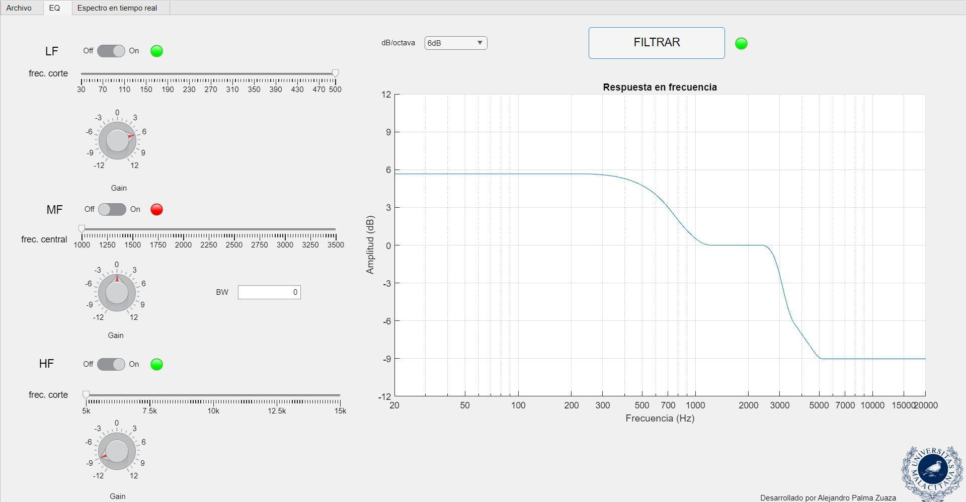
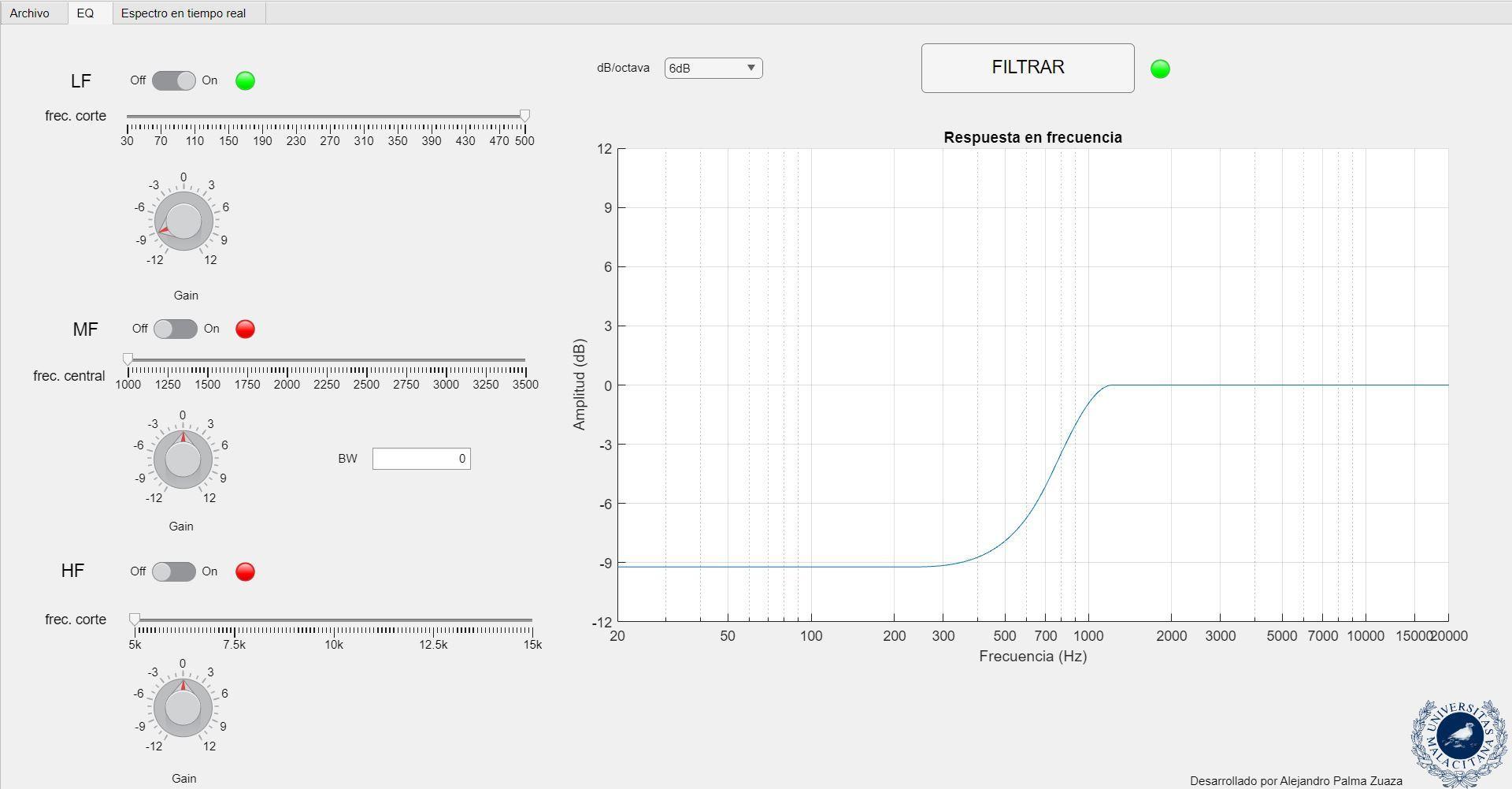
This is the main functionality of the app. It’s a 3-band parametric equalizer. Each band represents one frequency zone. The first one works in the Low-Frequency range, from 20 to 500 Hz. It`s a shelving filter, so you can choose the maximum cut frequency and the gain for that specific zone. The second one works in the Mid-Frequency range. With the slider you pick the central frequency, and you can choose the bandwidth as you want writing in the BW field. Basically, it’s a peak filter with the gain you set on the knob. The third one is for the High-Frequency range, and it’s basically the same as the LF one but in this one you peak the starting frequency, lasting until the end of the audible spectrum around 20KHz.

Once you set the parameters, you need to click on Filtrar, as it will draw the frequency response that you chose on the graph.

Now I will explain the two most difficult parts I faced during the development. I will start with how I drew the frecuency response

  1. Frecuency Response

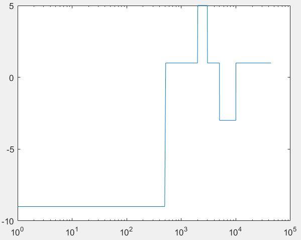
The first thing to do is create a frequency vector which will be the X axis. At first, I started with something simple by setting a piecewise function so for example if the LF zone was set with a cut frequency of 500 Hz, every point below that frequency would have the gain marked on the knob. Doing this, I achieved an ideal frequency response, so it was good as a first attempt. But the real challenge was to connect the 3 parts between them. To solve this problem, I defined one point between each part exactly in the middle between the end of one part and the start of the next one. Then, I connected the ending part of the first zone with the middle point -200 Hz. On the other side, I did the symmetric thing, linking the middle point +200 Hz with the starting point of the next part. The slope of these links is defined by the Pendiente field box. With this done, the remaining part was to connect the middle point -200 Hz with the middle point +200 Hz. As I had two points, I just calculated a linear function between them so now we have the two first zones connected. Doing the same thing but with the next two zones, now we have everything perfectly linked.

With this function defined, now we just evaluate the frequency vector in the previous function, so depending on the frequency it will have one value or another. This is the main code from that part.


puntomedio1 = (app.freccorteSlider.Value+(app.freccentralSlider.Value-(app.BWEditField.Value/2)))/2; %Primer punto medio
puntomedio2 = ((app.freccentralSlider.Value+(app.BWEditField.Value/2))+app.freccorteSlider_3.Value)/2; %Segundo punto medio
%hasta la el segundo elseif asignamos el valor del knob a cada zona
%frecuencial marcada
if abs(frec) <= app.freccorteSlider.Value
y = app.GainKnob.Value;
elseif (abs(frec) > (app.freccentralSlider.Value-(app.BWEditField.Value/2))) && (abs(frec) < (app.freccentralSlider.Value+(app.BWEditField.Value/2)))
y = app.GainKnob_2.Value;
elseif abs(frec) > app.freccorteSlider_3.Value
y = app.GainKnob_3.Value;

%A partir de aquí es para unir cada zona de forma correcta
%(LF, MF y HF)
%Desde el final de LF hasta el punto medio 1 -200 Hz
elseif (abs(frec) > app.freccorteSlider.Value) && (abs(frec) < puntomedio1-200)
%los max y los min son para que cuando la grafica
%tienda siempre a cero y no supere dicho valor por
%encima o por abajo.

if app.GainKnob.Value > 0
y = max(0, app.GainKnob.Value-app.pendiente*log2(abs(frec)/app.freccorteSlider.Value));
else
y = min(0, app.GainKnob.Value+app.pendiente*log2(abs(frec)/app.freccorteSlider.Value));
end

%Desde el punto medio 1 + 200 Hz hasta el principio de MF
elseif (abs(frec) > puntomedio1+200) && (abs(frec) < (app.freccentralSlider.Value-(app.BWEditField.Value/2)))
if app.GainKnob_2.Value > 0
y = max(0, app.GainKnob_2.Value+app.pendiente*log2(abs(frec)/(app.freccentralSlider.Value-(app.BWEditField.Value/2))));
else
y = min(0, app.GainKnob_2.Value-app.pendiente*log2(abs(frec)/(app.freccentralSlider.Value-(app.BWEditField.Value/2))));
end

%Desde el punto medio 1 - 200 Hz hasta el punto medio 1 +
%200 Hz, para unir el tramo restante.

elseif (abs(frec) >= puntomedio1-200) && (abs(frec) <= puntomedio1+200)
if app.GainKnob.Value > 0
valor1 = max(0, app.GainKnob.Value-app.pendiente*log2(abs(puntomedio1-201)/app.freccorteSlider.Value));
else
valor1 = min(0, app.GainKnob.Value+app.pendiente*log2(abs(puntomedio1-201)/app.freccorteSlider.Value));
end
if app.GainKnob_2.Value > 0
valor2 = max(0, app.GainKnob_2.Value+app.pendiente*log2(abs(puntomedio1+201)/(app.freccentralSlider.Value-(app.BWEditField.Value/2))));
else
valor2 = min(0, app.GainKnob_2.Value-app.pendiente*log2(abs(puntomedio1+201)/(app.freccentralSlider.Value-(app.BWEditField.Value/2))));
end

%Mediante valor 1 y valor 2 sacamos la pendiente de
%la recta que une ambos puntos
m = (valor2-valor1)/((puntomedio1+201)-(puntomedio1-201));
n = valor1-(m*(puntomedio1-201));

y = m*abs(frec)+n;

%Desde el final de MF hasta el punto medio 2 - 350 Hz.
elseif (abs(frec) > app.freccentralSlider.Value+(app.BWEditField.Value/2)) && (abs(frec) < puntomedio2-350)
if app.GainKnob_2.Value > 0
y = max(0, app.GainKnob_2.Value-app.pendiente*log2(abs(frec)/(app.freccentralSlider.Value+(app.BWEditField.Value/2))));
else
y = min(0, app.GainKnob_2.Value+app.pendiente*log2(abs(frec)/(app.freccentralSlider.Value+(app.BWEditField.Value/2))));
end

%Desde el punto medio 2 + 350 Hz hasta el principio de HF
elseif (abs(frec) > puntomedio2+350) && (abs(frec) < app.freccorteSlider_3.Value)
if app.GainKnob_3.Value > 0
y = max(0, app.GainKnob_3.Value+app.pendiente*log2(abs(frec)/(app.freccorteSlider_3.Value)));
else
y = min(0, app.GainKnob_3.Value-app.pendiente*log2(abs(frec)/(app.freccorteSlider_3.Value)));
end

%Desde el punto medio 2 - 350 Hz hasta el punto medio 2 +
%350 Hz, uniendo el tramo restante.
elseif (abs(frec) >= puntomedio2-350) && (abs(frec) <= puntomedio2+350)
if app.GainKnob_2.Value > 0
valor1 = max(0, app.GainKnob_2.Value-app.pendiente*log2(abs(frec)/(app.freccentralSlider.Value+(app.BWEditField.Value/2))));
else
valor1 = min(0, app.GainKnob_2.Value+app.pendiente*log2(abs(frec)/(app.freccentralSlider.Value+(app.BWEditField.Value/2))));
end
if app.GainKnob_3.Value > 0
valor2 = max(0, app.GainKnob_3.Value+app.pendiente*log2(abs(frec)/(app.freccorteSlider_3.Value)));
else
valor2 = min(0, app.GainKnob_3.Value-app.pendiente*log2(abs(frec)/(app.freccorteSlider_3.Value)));
end

%Mediante valor 1 y valor 2 sacamos la pendiente de
%la recta que une ambos puntos
m = (valor2-valor1)/((puntomedio2+351)-(puntomedio2-351));
n = valor1-(m*(puntomedio2-351));

y = m*abs(frec)+n;
else
y = 0;
end


  1. Filtering the signal

Now I will explain the signal processing I made to filter the signal with the frequency response that I explained before. In this part, there were several problems, but I managed to solve them. First, we need to isolate each channel in case that is a stereo file, so we process the signal in each channel. I decided to do block processing because if the user uses a long audio file, it would be very inefficient if I didn’t do that. I would also like to say that as I wanted to build it from zero, I didn’t use the filter matlab function. So, I used my knowledge in signal processing and did some research to do the process. First we need to set the vector frequency to the same length as the block we are processing. I decided to choose 2048 as the length of the block. So once this is done, we evaluate the vector with the piecewise function I explained before. Now we have the frequency response prepared, so now we need to prepare the signal block. To do that, I did an FFT to take it to the frequency domain. Now, having both signals in the frequency domain, we just need to multiply both ones, having the filtered signal. But now, we want to hear it, so it necessary to do an IFFT to take the filtered signal to the time domain. The problem doing only this, is that there were abrupt transitions between each block, and it sounded like the Audio_sin_solapamiento soundcloud link

To solve this problem, it was necessary to use windowing and overlap to the signal. Doing this, the start of the block will have a very little amplitude which will coincide with the peak of the signal, doing this process with each block. This is the code used to do the filtering:

%Extramos la señal del canal izquierdo y creamos el vector
%donde guardaremos el canal filtrado
canal_izq = app.signal_entrada(:,1)';
audio_fin_i = zeros(1, length(canal_izq));

%Si el audio es stereo, lo mismo para el derecho
if app.canales == 2
canal_der = (app.signal_entrada(:,2))';
audio_fin_d = zeros(1, length(canal_der));
end

%Establecemos el contador y el tamaño de los bloques
i = 1;
size = 2048;

%Creamos el vector de frecuencia con el mismo tamaño que los
%bloques
f = linspace(-app.fs/2, app.fs/2, size);

%Llamamos a la funcion para guardar en filtro la respuesta en
%frecuencia
filtro = filtrar(app, f);
filtro = movmean(filtro, 25); %hacemos un suavizado del filtro

cla(app.UIAxes2); %Limpiamos la gráfica

plot(app.UIAxes2, f, filtro); %Dibujamos la respuesta en frecuencia
filtro = 10.^(filtro/10); %Pasamos de dB a lineal

ventana = hann(size)'; %Aplicamos una ventana de Hann y
solapamiento = size/2; %solapamiento para que no haya transiciones bruscas entre bloques

while i < length(canal_izq) - solapamiento

if i > length(canal_izq)-size %Si es el bloque final hacemos lo mismo de antes pero con el tamaño restante
size = length(canal_izq)-i;
ventana = hann(size)';
solapamiento = size/2;
f = linspace(-app.fs/2, app.fs/2, size);

filtro = filtrar(app, f);

filtro = 10.^(filtro/10);

end

bloque_i = canal_izq(i:i+size-1) .* ventana; %Multiplicamos la ventana por el bloque
ei = fft(bloque_i); %Le hacemos la fft al bloque
sfi = ei.*fftshift(filtro); %Multiplicamos el bloque por el filtro centrado
bloque_i_filt = real(ifft(sfi)); %Le hacemos la ifft al bloque
audio_fin_i(i:i+size-1) = audio_fin_i(i:i+size-1) + bloque_i_filt; %Guardamos el bloque en el vector final

%Si el audio es stereo, lo mismo con el canal derecho
if app.canales == 2
bloque_d = canal_der(i:i+size-1).* ventana;
ed = fft(bloque_d, size);
sfd = ed.*fftshift(filtro);
bloque_d_filt = real(ifft(sfd, size));
audio_fin_d(i:i+size-1) = audio_fin_d(i:i+size-1) + bloque_d_filt;
end

%Actualizamos el contador para en vez de empezar al final
%del ultimo bloque, lo haga a la mitad para evitar la
%transicion brusca entre bloques

i = i+size-solapamiento;

end

%Asignamos toda la señal procesada a la señal filtrada
if app.canales == 2
app.signal_filtrada = [audio_fin_i', audio_fin_d'];
else
app.signal_filtrada = audio_fin_i';
end


Espectro En Tiempo Real

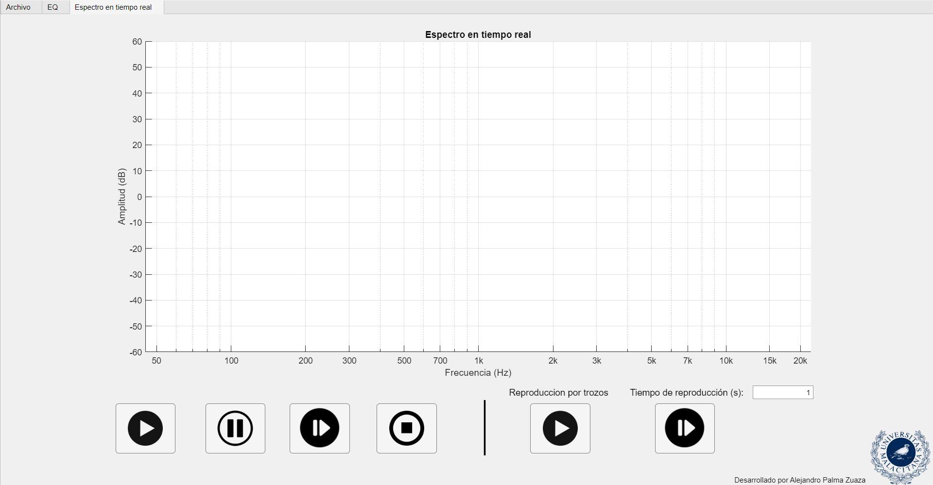
Eq_RTA_off.JPG
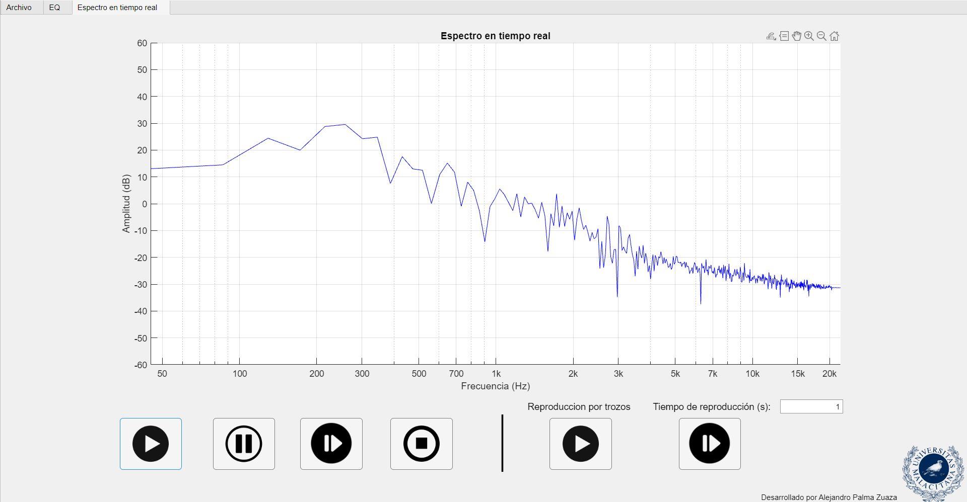
Eq_RTA_on.JPG

This page is useful to see the real time spectrum of the signal while the audio is playing. It has the same play, pause, resume and button as before. It also has two buttons where you can play little pieces of the signal. The duration of those pieces is determined by the “Tiempo de reproduccion” field value.

  1. RTSA

To draw the spectrum, I used a matlab function. Specifically, a property from the audio player which tells you what sample is currently playing. Knowing this, with a loop you can draw a small slice of the signal starting from that sample to make it fluent. The only step remaining to do is to do a FFT of that small part and then update the graph in every loop iteration. It’s very important to add the drawnow command in every loop, because is necessary to update the information shown in the plot. Here is the code:

function pinta(app)
cla(app.UIAxes3);

f = (1:1024/2)*(app.fs/1024);
linea_a_actualizar = line(app.UIAxes3, 'XData', f, 'YData', zeros(size(f)), 'Color', 'b');
nfft = 1024;
i = 1;
app.hline = xline(app.UIAxes, app.time(i), '--r', 'LineWidth', 1.5);
while isplaying(app.reproductor)

muestra_actual = app.reproductor.CurrentSample;
comienzo = max(muestra_actual-nfft+1,1);
fin = min(muestra_actual, length(app.signal_a_reproducir));

bloque = app.signal_a_reproducir(comienzo:fin);
transformada = fft(bloque, nfft);
transformada_a_pintar = abs(transformada);
transformada_a_pintar = transformada_a_pintar(1:nfft/2);
transformada_a_pintar = 20*log10(transformada_a_pintar);

set(linea_a_actualizar, 'YData', transformada_a_pintar);

drawnow
end
end


  1. Play & Resume buttons with a predefined playback time

The last thing I would like to explain is the two right buttons. These ones are used to play little parts of the file. For example, if you write 2 on the Tiempo de reproduccion field box, it will play only 2 seconds. When you play one of those buttons, a timer is activated lasting the amount of time you choose. When this timer finishes, it has attached a function which is a pause in the audio player.


Proyect Demostration
Tutorial EQ

To finish with, there is a video of me explaining how to use it and some audio file before (Sin filtrar) and after the filtering (Sin graves). I hope you liked it.