6 Axis Robotic Arm With Generative Design and Deep Learning
by krishandjoe in Circuits > Robots
7212 Views, 99 Favorites, 0 Comments
6 Axis Robotic Arm With Generative Design and Deep Learning

Hi, This Instructable is a collaboration between Joseph Maloney, 16 years old, and Krishna Malhotra, 15 Years old. Joseph wrote the generative design section of the Instructable, and designed and built the arm. Krishna wrote the software section of the Instructable, all the code for the arm, and assembled the electronic components and wiring. This Instructable will teach you how to utilize generative design and neural networks to make an optimized robotic arm. Furthermore, it will cover how to develop your own deep learning models and the general and mathematical theory behind the complex neural network algorithms.
Generative design is a way of using a computer to optimize 3D models. It can be used to make parts lighter, stiffer, and with less material than previously possible. It works by applying loads to parts and running a simulation. Then, using the results from the simulation the computer iteratively adds or removes material wherever necessary. Constraints such as manufacturability and target weight can be set to achieve the optimal design for your application. In this Instructable you will learn the basic functionality of fusion 360s generative design workspace. These skills can be utilized on almost any design and can help you take your modeling skills to the next level.
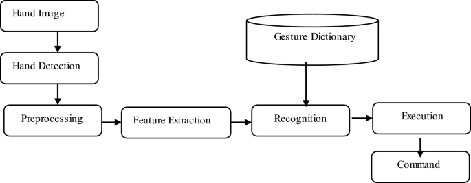
Furthermore, using an advanced, novel recurrent neural network, a deep learning model implemented from scratch using the TensorFlow library in Python, demonstrated the capability of interpreting audio into text, and listening for key tokens (words). This was then translated onto the robot, enabling a user to simply command the robot to do something and that to be translated on the robust, optimized 6 DOF robotic arm. For instance, one could just say, “Get me that banana.” The audio goes through the recurrent-neural-network, extracts key words and then a predefined movement is activated on the robot. In addition, through a more beginner-friendly design, using the mediapipe deep learning tools and computer vision libraries, the robot is capable of mimicking hand movements done by the user allowing for a user to control the robot simply by using hand gestures. Finally, once again using the beginner-friendly tools, a computer vision model was used to track objects of a specified color and using angular calculations, the robot is able to orient itself towards the object and successfully pick and place it.
Supplies
The software you will need for this project is,
- Fusion 360
- Ultimaker Cura - or other slicer
- PyCharm (or other Python IDE)
- Arduino IDE
The supplies you will need for this project are,
- 3D Printer (Prusa I3 MK3s+)
- PLA filament or other stiff filament
- 6x Servos (LDX-218 & LD-1501MG servos)
- Arduino UNO
- Male to Male Jumper Wires
- 2 18650 Lithium Ion Batteries + Battery Pack with wire connections (+ and -)
General Design
This step will be briefly covered due to the fact that this instructable is not about overall design and rather is about utilizing AI in design. With that in mind, Here are some key tips I can give for the design.
Inspiration: Look at some images of other robotic arms. Small arms in particular usually have compact and rigid designs.
Rigidity: Keep all of the degrees of freedom as rigid as possible. This can mean using bearings on joints that have more force applied to them. I highly recommend a bearing on the first degree of freedom as a minimum because the weight of the whole arm is applied to this joint.
Servo selection: Don't use too small of servos for your arm. Double check the torque of your servos and make sure that they can move at a reasonable speed.
Weight: The goal of generative design in many cases is to reduce weight. Lighter robotic arms will be able to move faster and be more precise.
Preparing Models Optimization
For this demonstration I will be walking you through the process of optimizing one part in Fusion 360. The same principles can be applied to all the parts in the design of your robotic arm.
Picking a part to optimize: You are going to want to choose a part with some margin to improve upon. In many cases the point of generative design is to reduce weight and volume. In this example we will optimize an already made part as opposed to creating the part completely through generative design. Start with a part which is too strong, leave material to be removed on your part. Make sure that your design is final in terms of hole placements and clearances. I recommend starting with a simple and consistent part. The part must be a component. Any areas of your part that you do not want to be affected by the generative design process, such as screw holes, must be separate bodies.
Topology optimization vs generative design: Topology optimization is where you start with a part which is "too strong" and iteratively optimize it to bear a certain load or set of loads. Generative design is a broader term which isn't necessarily constrained by a starting body. In many cases generative design does not need a starting body at all.
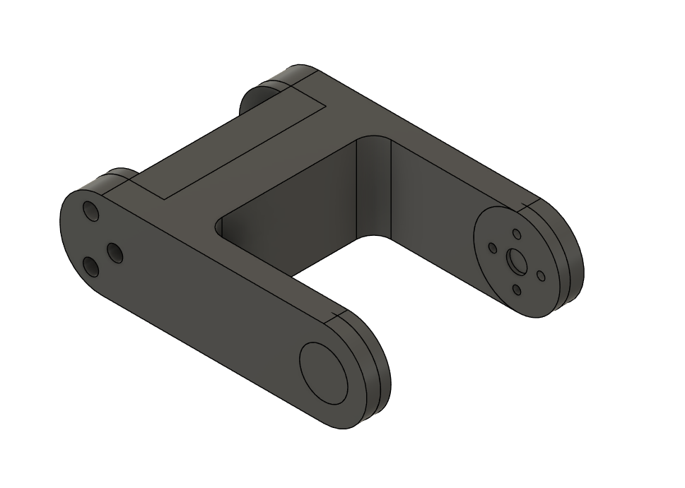
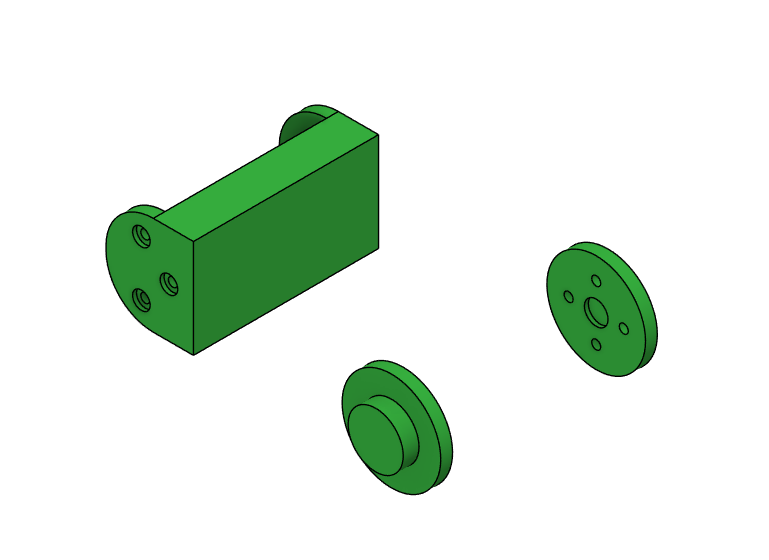
Simulation specific CAD: To utilize generative design, like I will be doing in the example, you do not need to design your whole part. You simply need to design any areas of the part that must exist for the parts functionality. In the example above, I designed the holes and servo-mounting points as separate bodies so that in later steps they can be set to preserved geometry. I also included a body that would work for the application. This is simply for visualization and it does not affect the simulation.
Assigning Materials, Objectives, and Manufacturing
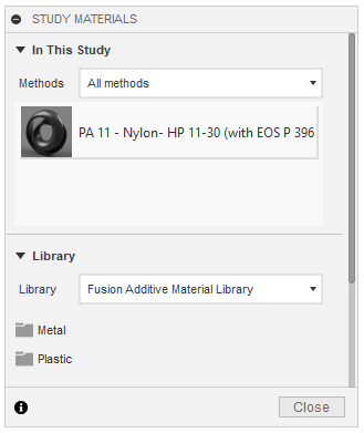
Assigning study materials: To assign a material, click on the "study materials" option in the top bar. Then drag and drop your material into the top section of the wizard. Unfortunately, fusion 360 does not have a study material for PLA or other 3d printing materials. After comparing the material properties of the plastics that fusion does offer, the one most similar to PLA is PA 11 - Nylon. You can either just run your generative design with this material or create your own material for PLA. This can be done by editing the properties for a material, and changing them to the properties of PLA.
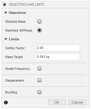
Setting up objectives: To set objectives, click on the "objectives" option in the top bar. Here, you can either choose to minimize mass, or maximize stiffness. Minimize mass will, using the material and loads you define, make the lightest part possible. Maximize stiffness on the other hand will take a target mass and try to achieve that mass with the highest stiffness possible. For my design, I chose to maximize stiffness because it gives more control over the final mass of your part.
Safety factor: The safety factor is a way to define how close the design can get to bending, or breaking when subjected to the applied loads. A safety factor of less than one means that a failure will occur. The safety factor is defined under the objectives wizard. I recommend setting this setting to anything between 1.6 and 3. In my design I chose a safety factor of 2.
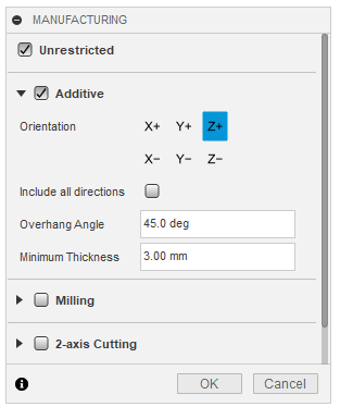
Manufacturing constraints: Manufacturing constraints are a way of ensuring the parts that are outputted by the generative design process are manufacturable. For 3d printing, this is not much of a concern. There is an "additive" constraint where you can set the max overhang angle. However, you can just print your parts with support material and this is not too much of a concern. I recommend setting the manufacturing constraints to unrestricted. This also allows for the generation of more unique shapes and stronger parts.
Assigning Preserve Geometry
Generative Design workspace: To enter the generative design workspace, select it from the options in the top left as you would for rendering. After entering the generative design workspace, you will be prompted to create a study. Select "create study" and you are ready to go.
Selecting Preserve geometry: To select preserve geometry, select the "preserve geometry" tab under the study you created. Then select all the bodies that you don't want to be modified by the generative design process. Keep in mind that these have to be created in the modeling process as bodies under the component you are optimizing.
Assigning Obstacle Geometry
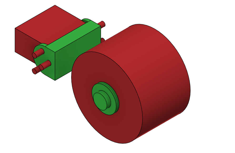
Obstacle geometries are modeled parts that the generative model is not allowed to generate in. I recommend that you use obstacle geometry to preserve any mounting holes and servo clearances. Obstacle geometry can also be used to force the model to generate into a more appealing shape. It can be assigned in the same way that preserve geometry is assigned. Once assigned, obstacle geometry appears in red. In the example above, I used obstacle geometry to stop the generative model from generating in the mounting holes, and to allow for 360 degree clearance around the servo.
An alternative to using obstacle geometry is using a starting shape and setting the mode to only remove material. Both methods work well and in most cases it comes down to convenience.
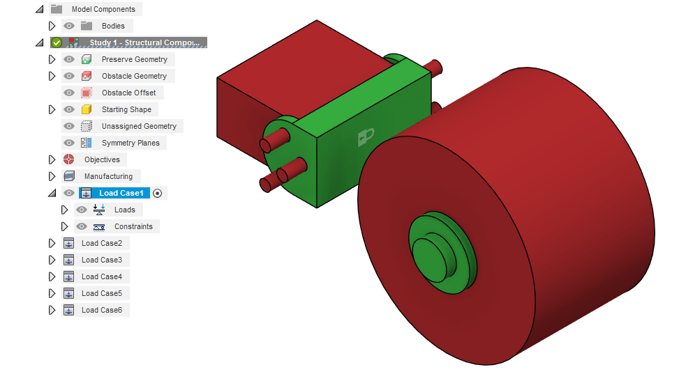
Load Cases
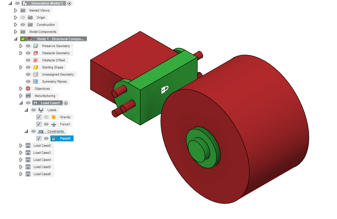
A load case is a set of constraints and loads that are applied to a simulation model. Each load case stores a set of structural loads and a set of constraints. They appear as a node in the Browser and can be cloned and created. You can have as many load cases as you want but the fewer the better. Less load cases speed up the simulation and make the whole process simpler. Load cases can be activated in the same way as components and any added constraints or structural loads will be created under the activated load case. The best time to create a load case is when you need to incorporate 2 or more forces into your part, and you don't want them to interfere with each other. For example, if you want to simulate a part with two different forces but the forces would cancel each other out, then you need to use two load cases. Remember to redefine your constraints when creating new load cases. In the example I gave, and in many other cases, it is faster to clone the first load case and then change the structural load. In the part above I needed to use 6 load cases in total and this resulted in a simulation time of around 15 minutes. Of course, simulation time relies on many factors and this was a relatively simple part.
Constraints
Constraints allow you to define how your model reacts to the forces you apply. Constraints are assigned to the model to stop it from moving in response to applied loads. In this instructable, I will not be covering all of the constraint types and in most cases you will not need to use more than simple fixed constraints.
Assigning constraints: To assign a constraint, simply activate a load case and under the design constraints tab select structural constraints. Then select the face or face group that you want to constrain. Finally there will be additional options like which axis are to be affected by your constraint. Choose whichever options meet the needs of your constraint.
Fixed constraints: Fixed constraints lock 1 or more axes of movement for a face. By default, fixed constraints lock all three axes and they are the most common type of constraint to use in generative design. For simplicity let's consider that all axes of the constraint are locked. A fixed constraint will not let the face move or stretch in any way during the simulation.
Frictionless constraints: Frictionless constraints constrain the movement of a face to an extension of that face. They do not have any additional options and are used in applications where you want to constrain a part while still allowing for movement in a certain axis. A frictionless constraint will let the faces move or stretch in any way as long as they remain in the same plane or arc and do not interfere with other constraints.
Structural Loads
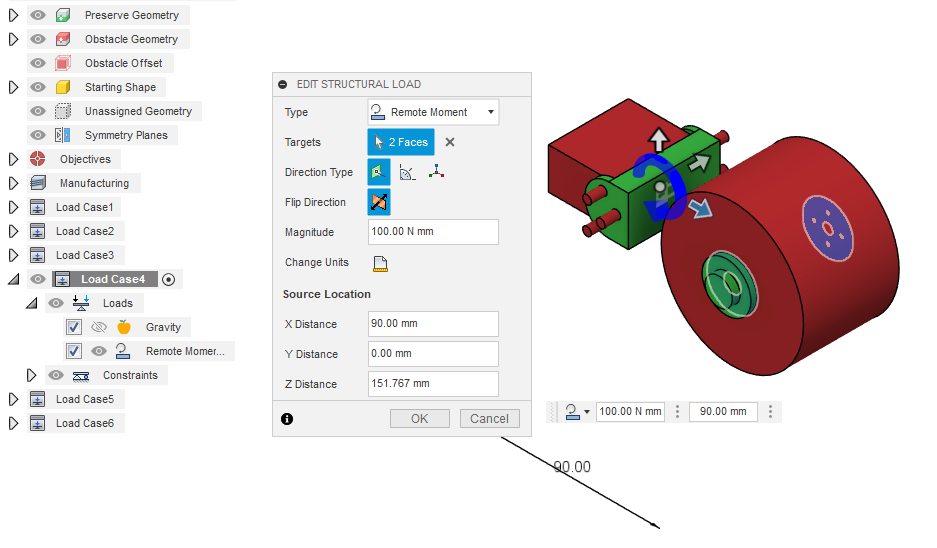
Structural loads are the forces applied to your part during the simulation. The generative design model will be optimized to achieve the objectives, which were defined earlier, and make the part as strong as possible under these forces. I will not cover all the different types of load cases and in most cases you will only need to use the ones mentioned in this step.
Assigning loads: Loads are assigned in the same way as a constraint. Simply activate a load case and under the design constraints tab select structural loads. Then select the face or face group that you want to apply to load to. Additionally, there will be options like the direction type. The direction type is how you define which system is used to define the direction of the force. It is necessary in all types of structural loads except for bearing loads and pressure loads. Use whichever direction type is simplest for the application.
Forces: Forces are exactly what they sound like. A constant force applied in a certain direction. The direction can be defined through the direction type. The force is set by inputting a value into the wizard. Remember to keep in mind the material for your application when setting forces.
Moments: Moments are torque forces set around an axis. They are defined through a direction type like forces. Although, due to the fact that the force is applied around an axis, the input for moments is in Newton meters or similar depending on your unit preferences.
Remote forces and moments: Remote forces and moments are a way of moving the center or axis of the force to a specific area outside of your part, or to anywhere in space. They can be used to more realistically model the stresses on your part.
Symmetry
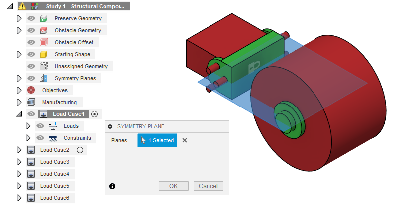
Symmetry can be taken advantage of in generative design in the same way as in conventional modeling. When deciding whether to use symmetry you need to consider the forces applied to your model in earlier steps. If the preserve geometry and forces are equal across a plane then it is recommended that you set that plane to be a symmetry plane in the simulation. Symmetry can also be utilized to ensure that your part is symmetric for visual purposes.
Pre Checks and Generation
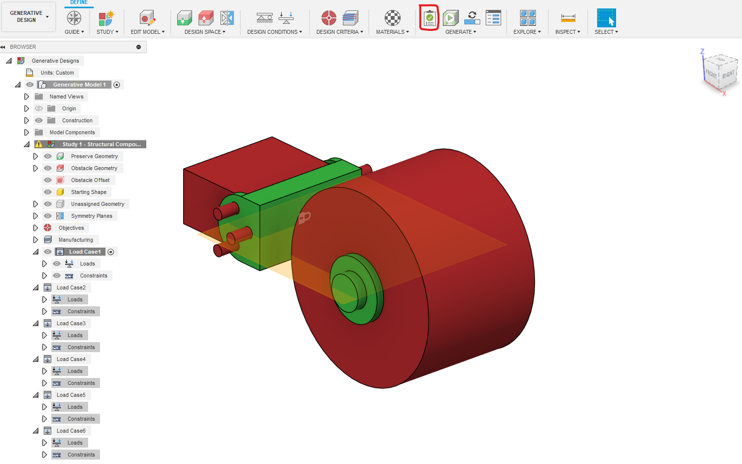
In this step, you will finally be able to see your results. First, however, you need to make sure that the Pre-Checks tool, as circled in red, is a green checkmark; Similar to the one shown above. If instead it displays a yellow or red warning sign, then you need to review the previous steps. Finally, once everything looks good, click the generate button. The model will take, depending on the complexity of your case, anywhere between 20 minutes and 3+ hours. The operation however runs on the cloud so you can use your computer or even fusion 360 for something else. Once outcomes start generating, you can see them through the explore option. There will be one different outcome for every material assigned and each outcome will have many iterations. You can preview these outcomes but wait until the whole generative design process is complete before exporting them.
Creating Designs From Results
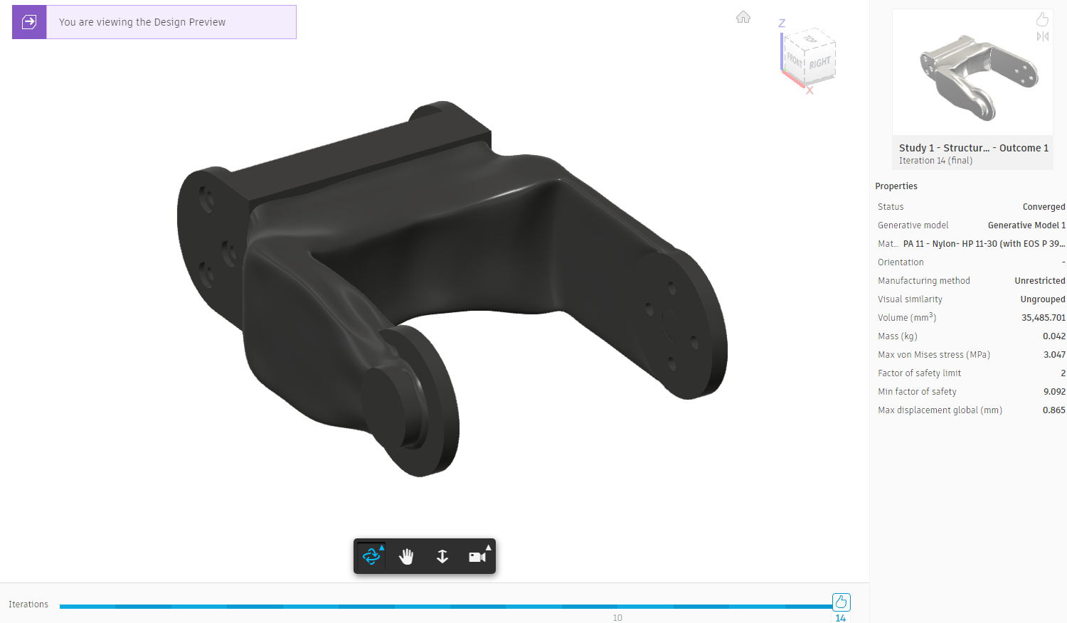
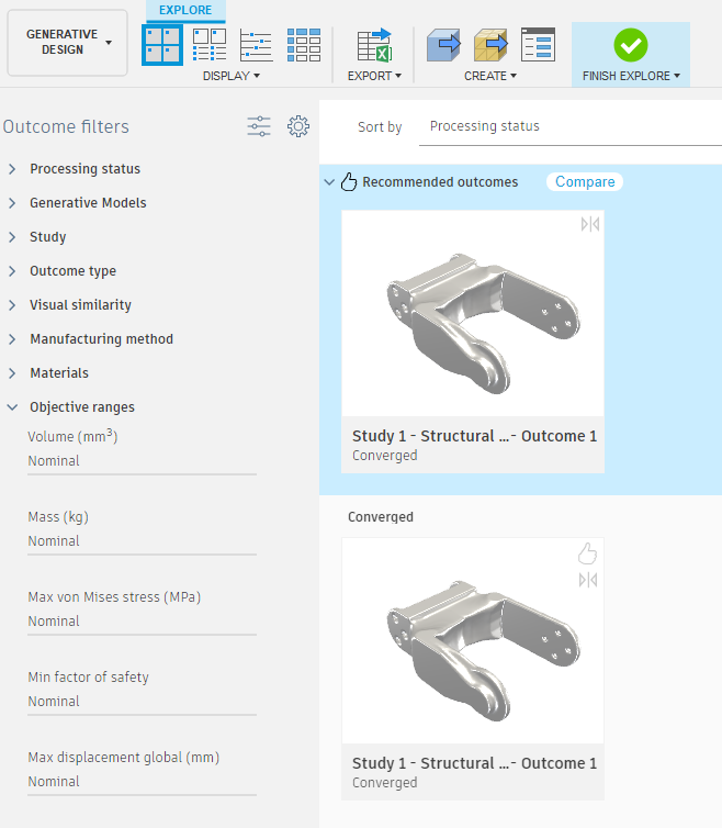
The final step in the optimization of parts is creating designs from your results. First go to the explore tab of the generative design workspace and select the version that you want to build a design from. You will only have one option if you simulated with one material. This screen gives you the option to view the stresses on your part with a gradient by selecting the option under display. If you are going to directly print your part then you can directly export it as a mesh through the option under "create". More likely, however, you will want to import your finished part back into your original arm file. In this case you can create a design from your part by selecting "design from outcome" under "create". Once The design is generated it will create a separate model. You can edit this model and make any tweaks you need to like changing hole sizes. You can also Go back in the timeline and directly change the shape of the generated model as a T-Spline. Once you are happy with the final design, save it and import it back into your design. If you import it under the same component it was created from then you might not have to redo the joints, but in most cases you will. Congratulations! you now know how to use the generative design tool.
Programming Resources
We will use google colab. If possible, their $10 payment for 100 compute units allows for longer session durations and faster GPU processing. We will be making a complex, full-scale NLP Deep learning model in it so it may come in handy. THIS IS NOT MANDATORY BY ANY MEANS. If your computer has a GPU already, simply use PyCharm or run it by CPU if you do not have one (this may take a while and is not recommended, I recommend google colab in this case.
To download PyCharm, visit https://www.jetbrains.com/pycharm/ and follow below video instructions

Frameworks and Libraries
First, go onto google colab and open up a new project. Connect to any availale GPU's. Keep in mind that if you do not have colab pro, you may need to work quickly as the session closes down after a little while.
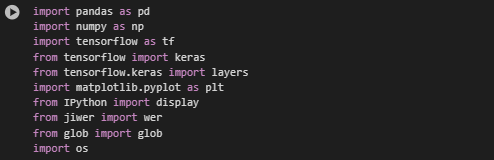
For this chapter, we will be using the TensorFlow/Keras Libraries. These libraries are powerful tools that will allow us to develop a functional deep learning model. I am using google colab due to their fast GPU’s, (meaning less training time) and the already included libraries. Simply, just import the libraries as shown:
Data Loading
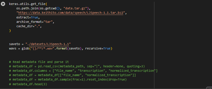
Next, we need to download a dataset for our model to train on. The best candidate for this is the LJSpeech1-1 dataset which contains thousands of .wav files of volunteers reading non-fiction books. We will train our model to understand the large variety of words and use it to have our robot do commands when prompted by a recognized word. We can download it simply by giving the URL as shown below. Then, we will define the vocabulary that the model will be able to understand. This refers to all the letters in the alphabet and special symbols. Additionally, we will define a Keras pre-built function to convert raw outputs of the model into characters for later.
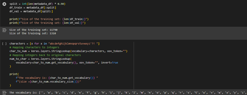
Lets print out some information regarding the data size and the character parameters:
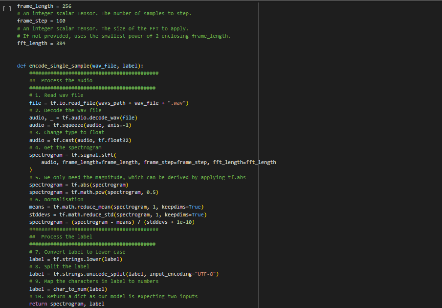
Data Processing
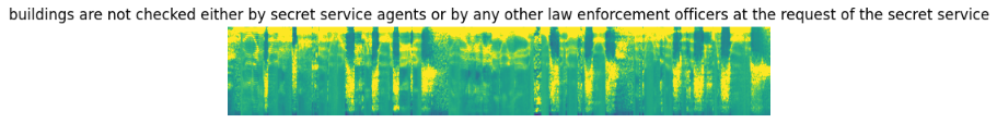
Now, we need to process our data into a form our model can handle. This can be accomplished through spectrograms. Spectrograms are another representation of an audio wave and can have deep learning algorithms applied to it because it’s similar to a normal image. But to have this be processed by the model, we need to convert the spectrogram into tensors. Think about tensors like the neurons in your brain. For the entire brain to work, process, and do its functions, it requires individual neurons. Tensors are the neurons for the whole deep learning model and each of them does a specific calculation. They are processed in the CPU or GPU. TensorFlow can handle them very well and includes pre-built functions to do this conversion as shown below. All the code is doing is converting the file it reads into spectrogram tensors and normalizing the data into a normal distribution for further processing.
Spectrogram Output:
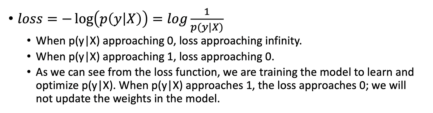
Now, we must create a training and validation split. Our model will be trained on the training dataset and to calculate error for improvement, it will use a validation dataset to verify the prediction it outputs.
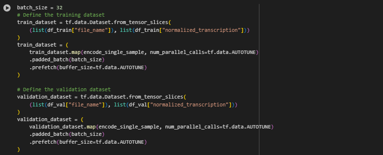
Model Architecture
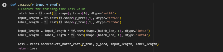
Before we create our model, we need to define a loss function. There are a variety of loss functions but they all have the same goal; minimize loss. A loss function will calculate a model’s performance based on the actual label (in our case word) and the prediction. Then this will feed feedback into the model for it to correct its incorrect outputs and further optimize the outputs. For sentence data like the one we are using, CTC loss is the most efficient. Connectionist Temporal Classification (CTC) is a type of loss function we will use to evaluate our model. Any other loss function may not be able to provide accurate feedback due to the sophisticated nature of word classification. In sum, CTC loss will be given a label and a prediction from the model and will calculate the negative log likelihood of it being correct.Then the model will use this to further optimize its output. CTC is the loss function of choice because it can handle multiple inputs and multiple outputs. Most model types and loss functions expect a single input and a single output but CTC expects multiple inputs and outputs, thus allowing us to optimize our loss. The equation looks like this:
Now let's construct this in code. Luckily, TensorFlow already has this mathematical function built in so we just have to initialize the loss function as such:
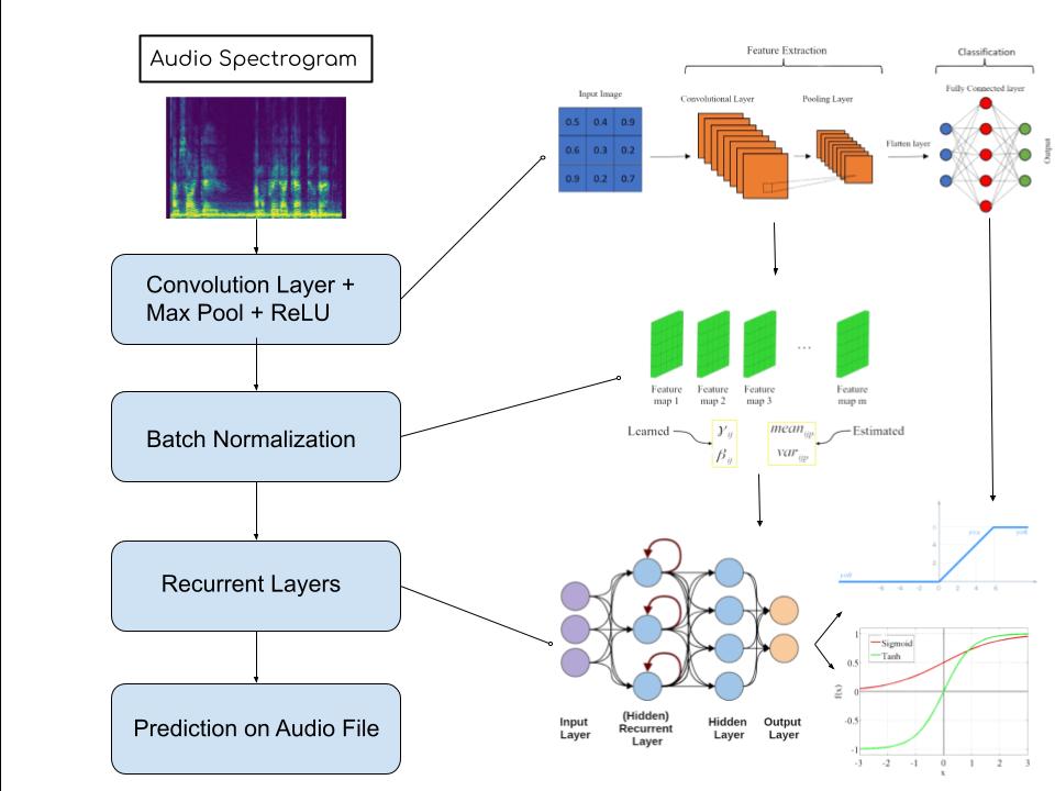
Now we must construct our model. First, we will segment the words and characters from the actual sentence for our model to not have to worry about the confusing English grammar but rather formulate characters based on what the input sound is. This can be done using a convolutional neural network (CNN). As mentioned before, a spectrogram is almost like a sound image so we can teach the CNN what characters and words are like based on the spectrogram images.
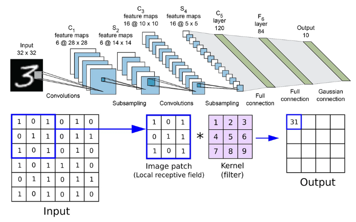
Convolutional Neural Networks (CNNs): In sum, a convolutional neural network will input an image and extract an n number of features. Then it maps these features to smaller or larger pixels (depending on the model architecture) through a process called max pooling. Within each of these steps, their data is stored in neurons and a specific mathematical equation is performed on them. Over multiple layers, the model learns to categorize the pixels of an image into the specified outputs. In our case, these are the characters. Finally, output tensors in a 2D format are flattened into a single 1D array through a process called linearization. The diagram below refers to a model that can classify numbers. I recommend watching this animation to gain a better understanding: Convolutional Neural Network Visualization by Otavio Good
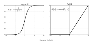
ReLU is a common technique that we will be using in our model. It prevents negative values from being processed which is useful for identifying junk and extreme, useless outputs. Another one we will use is called softmax which will convert our raw outputs into probabilities we can understand. For instance, instead of outputting a bunch of numbers only understandable by a machine, softmax, in our case, will predict the characters being said as probabilities such as a user saying a may yield a 99% probability once the word ‘apple’ is said. These two methods are widely known as activation functions and are fundamental to deep learning. Here is what the graphs of both look like:
Now we can implement this in the code. The code applies two convolutional layers including a ReLU activation after each
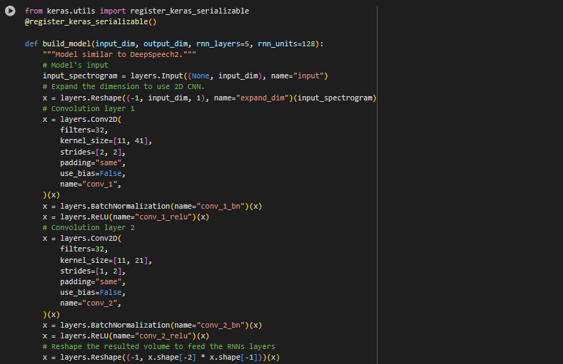
(Note: To save model you must add @register_keras_serializable() above model building)
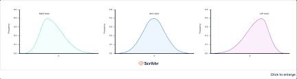
You will notice we implement “Batch Normalization.” Batch Normalization is a process in which the outputs of a model become normalized. The outputs may be skewed and incorrect so Batch Normalization subtracts the batch (previous output) mean from it and divides by the standard deviation. An example graphically is shown above the code snippet. The graph on the left shows a raw output while the graph on the right shows a normalized output.
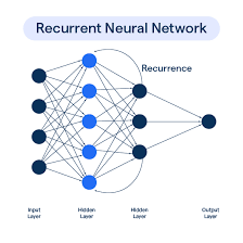
Recurrent Neural Networks (RNNs): Following the character and word segmentation performed by the CNNs, it is crucial for our deep learning model to be able to classify the words and letters specifically. This can be achieved through a Recurrent Neural Network. Most models like the CNN symbolized above strictly moves forward in its processing. It goes from the start neuron to the end neuron strictly forward in what’s called a forward pass with a single backwards pass. RNN’s on the other hand use a process called backpropagation through time (BPTT) after each tensor (remember these are the neurons) which allows the model to remember past information. This allows for sequencing data like sentences and words because for example, if your model is given the word “Appl”, it can use the backpropagation to remember “A”, “p,” “p,” “l” leads to the word apple and make a prediction. This is especially useful in our model because audio may become easily distorted so being able to make inferences as such is a key tool. In summary, think about RNN’s like a normal neural network, but after each section, the model uses the stuff it just learned to enhance its predictive nature.
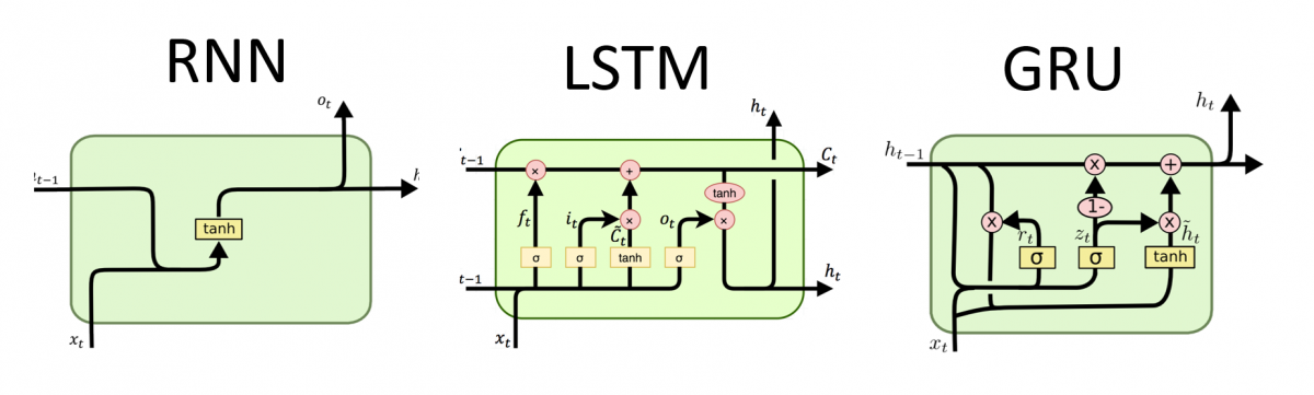
However, an issue with RNN’s is that when it undergoes its backpropagation algorithm, it calculates gradients to be able to minimize the loss function discussed earlier. When doing so, a model may overshoot leading to enormous gradients or exponentially decrease, deteriorating the model’s accuracy. This is a problem specifically with RNN’s because since they use backpropagation through time, the gradients have nowhere to escape the model’s training cycle causing accumulation that leads to giant values. Thus, we use a method called Gated Recurrent Units, or GRU’s. GRU’s are a variant of the traditional RNN. The processing and architecture of the models are identical, but GRU’s act as gates, allowing gradients to escape. GRU’s know when to let out the gradients (once accumulation starts to occur) and when to keep them for optimized loss calculation. Another similar way is called LSTM, but they are too computationally expensive, potentially causing model training to take days.
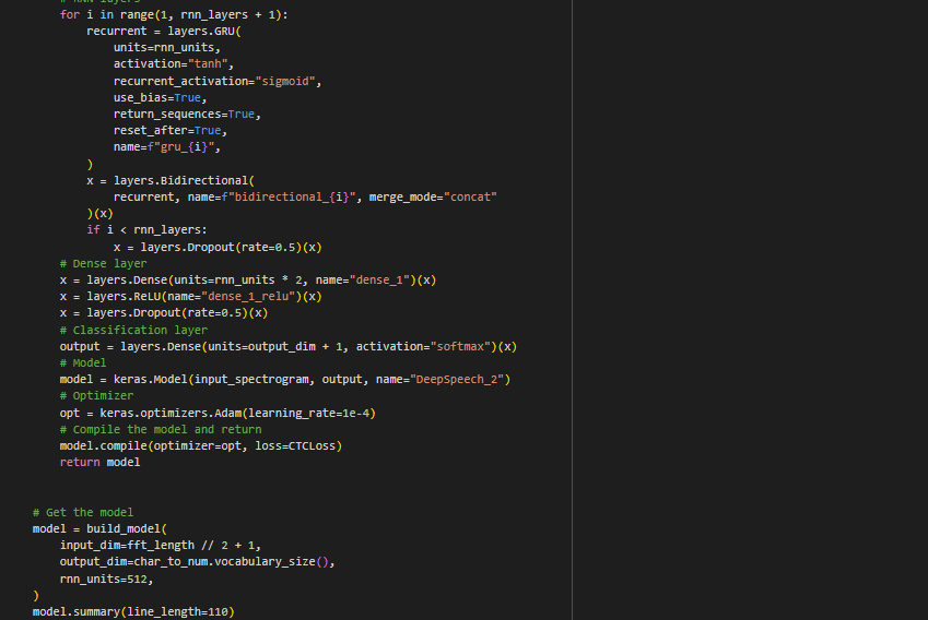
Now, we can implement this in code. We will take the output of our convolutional model (x), which has been normalized, and input it into a GRU loop. This way, the model undergoes multiple BPTT cycles every training cycle (epoch)
As we iterate through our RNN/GRU cycles, we define a bidirectional layer to allow for the forward pass portion and recurrence portion. We then condense (Dense) the output down to the units calculated by the RNN to be able to make an output and apply a ReLU and Softmax activation function.
This is what our model looks like:
Model Training
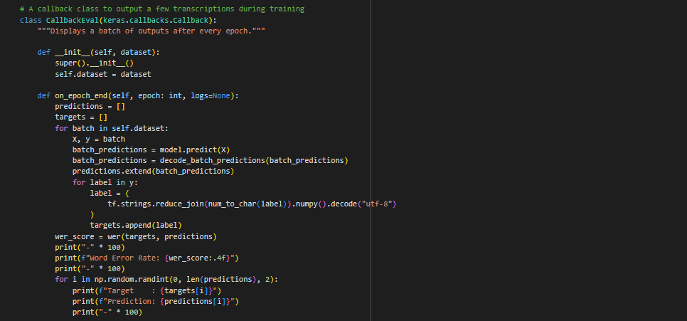
Model Outputs and Decoding: Before we go ahead and begin the training process, it is important to develop a way to decode the model’s output (gibberish tensors). Additionally, during training it is useful to know how the model is performing a lot only by metrics like the CTC loss, but actual predictions from the training cycle. To do this, we will use Keras’ utilities to convert the prediction to numbered outputs and the previously defined function in Step 14 to convert the numbers to characters.
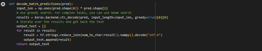
So now that we have a way to decode the output, we can develop a mechanism to make predictions after every other training cycle (epoch). The code simply uses Keras’ in-built model.predict(x) function to retrieve the predictions and then passes that to the decoder we just defined.
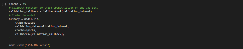
Now we can finally train the complex model on the dataset. This is very easy to implement using TensorFlow, as you can just use model.fit() to train it. Then we will save it as a .keras file.
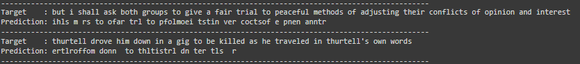
This is what epoch 1’s predictions looked like:
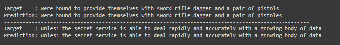
This is epoch 45, a significant improvement:
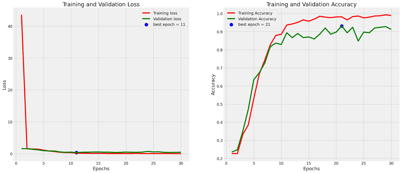
Below is the final graphical data of the model training. We can see loss was minimized and the accuracy was above 95%
Robot Implementation
Now we use the model to make predictions on the voice saved in a file. Then we can use some simple algorithms to determine key words in the output and activate pre-defined functions for the robot to do. This will be done in PyCharm as it will allow us to do serial communication easily.
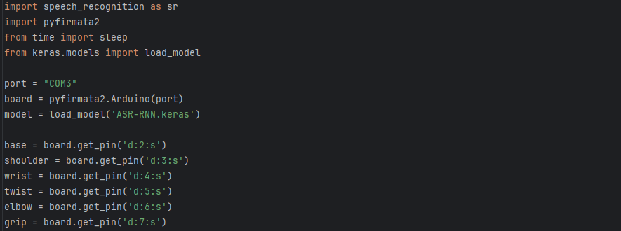
We will utilize the PyFirmata library to do this. First we will make the necessary imports and set up our environment. We define where on the Arduino board the motors are and the serial port. In my case, the connection is ‘COM3.’
Before we give out robot commands, let’s make the circuit and prepare the Arduino board. If you have not already, install the Arduino IDE from https://www.arduino.cc/. Now follow the diagram below to wire the robot. Pay close attention to the provided notes as you may damage parts if not read thoroughly.
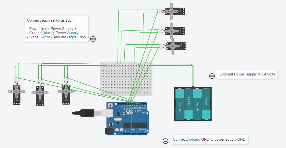
- Connect Grounds of Arduino and External Power Supply
- Make sure Black and Red wires go to their corresponding places
- Power supply does not exceed 9V and is over 7V
Now, upload this code to your Arduino and plug in your power supply: https://github.com/Krish-mal15/Instructables-Made-With-AI-Contest-Code/blob/main/Object-Detection/PyFirmata-Object-Pick-and-Place.ino
This is the PyFirmata protocol for the Arduino to recognize the commands. This is the only code that will be implemented on the Arduino in the rest of this so keep this code uploaded. Follow the below steps for all the chapters:
- Upload GitHub code at link above to Arduino
- Plug in external power supply
- Plug Arduino into computer
- Run code in PyCharm
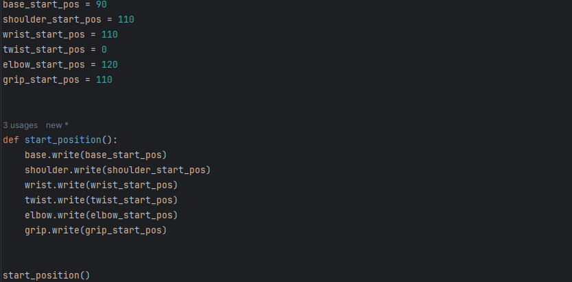
First, send a signal to our robot to prevent jerky movements (start position)
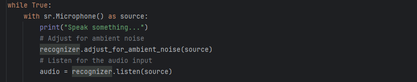
Moreover, we will use google speech library to develop the audio in the necessary spectrogram format. It automatically does this as such:
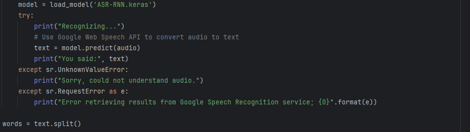
Now we can load out model and make a prediction from the audio
Then, we will define the pre-built commands for our robot. You may reference an example from the GitHub code linked at the beginning on this Instructable.
Finally, let's call the functions based on the recognized words:
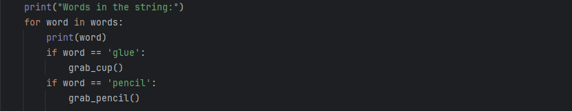
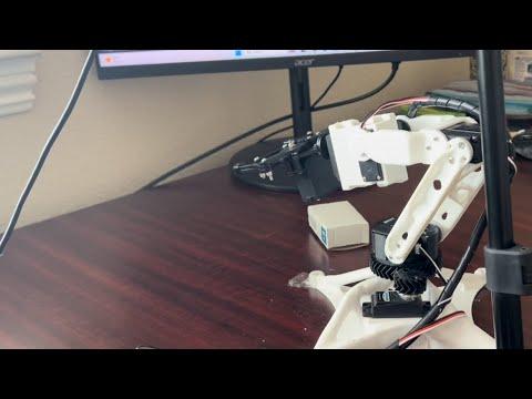
Congratulations! You made a deep learning recurrent-convolutional neural network for the daunting Automatic Speech Recognition task and learned how to control an Arduino with Python! Here is the robot in action:
Voice Recognition Demonstration
Computer Vision Object Tracking
For a more beginner friendly approach, we will implement an object tracking element to our robot. This will work by detecting a color of choice, automatically aligning to the object and picking it up and placing to a predefined spot.
Imports and Global Variables
First, we import our libraries. We define a ColorModule from cvzone which will allow us to track colors very easily. Then we establish our PyFirmata connection like before.
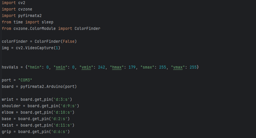
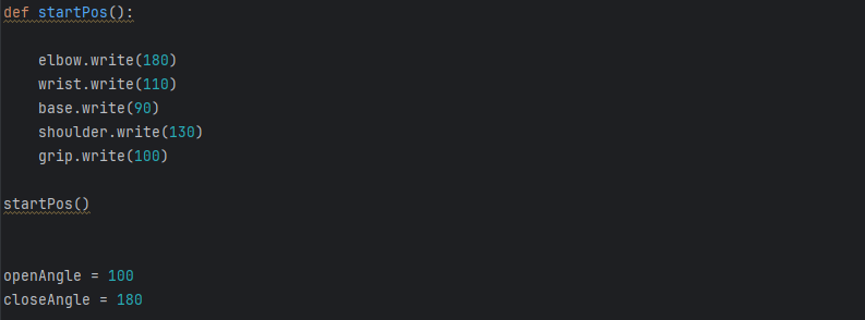
Robot Configuration & Commands
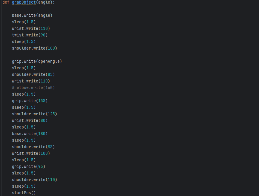
We first define a start position for the robot. Then we create a function to make the base turn to a given angle and to execute a command for the robot to go down and pick up the object.
Computer Vision
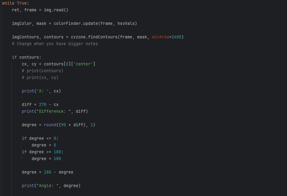
Then we use the cvzone function to retrieve the contours from the frame and get the coordinates. Then, we add a couple safety features not letting the angle exceed 180 degrees or under 0 degrees. Furthermore, due to the design of the robot, we must invert the angle subtracting it from 180. The tracking works by accounting for “error” between the center of the camera and moving the robot to adjust for error.
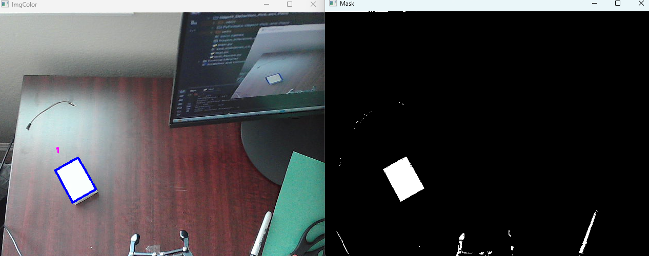
The computer vision uses opencv’s functions for contour detection. Contours are just the object of a certain color’s outline. What the code is doing is putting a mask over the image as it detects pixels with a certain HSV value. That is why we specify that value as one of our global variables so we can tell the computer vision library what pixels we want. Then we lay out the detected pixels over the image and use the center of the contour to use as coordinates. Most of this is handled in the cvzone library. This is what the output looks like. We give the model HSV values to detect white and provide a minimum area. This ensures no background tiny white objects are detected. We then overlay it onto the real image to look like this:
The angle calculation works by the following
- Detecting x position of object (contour) relative to screen (between 0 and 540)
- Finding difference between the midpoint of the screen (270)
- Adding an offset of 90 made by just testing
- Not letting angle exceed 180 or become negative
Interface
Lastly, we add a feature to retrieve an input from the user asking if it should grab the object. If the user inputs ‘y’ then the base will align to the angle calculated to the object and then perform the grab function defined earlier. This is what the computer sees:
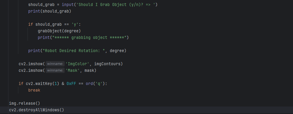
Finally, set up a webcam above your working plane with the robot positioned in the middle and mostly out of frame. Then, upload the code and watch computer vision do it's magic!
Object Tracking Demostration

Keep in mind, this was a very basic demonstration. You can make it do all sorts of things such as moving items off of a conveyor belt.
Computer Vision Hand Tracking
We will now implement a feature for the robot to mimic the movements done by our hand.
Overview
Now that PyCharm is downloaded, you can set up your project virtual environment. Simply create a new project and then install the following packages:
- mediapipe
- opencv-python
- numpy
- PyFirmata2
- cvzone
Mediapipe is a huge library containing pre-trained deep learning models for various applications. In our case, we will be utilizing the hand-tracking features. From there, we will use that model and run it on each frame of a live video captured using OpenCV. Finally, we will track the movements of the hand relative to the screen and translate it into actual robot movements. For more details, see: https://developers.google.com/mediapipe/solutions/vision/hand_landmarker/python
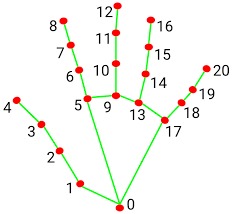
Google has developed a deep learning model trained on thousands of hand images. Through more complex algorithms, the detector is capable of pinpointing specific landmarks on the hand which will come useful when controlling the gripper of our robot.
This is what the landmarks look like:
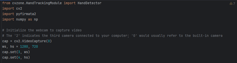
Libraries Video Capture
First, we import the necessary libraries and set up our OpenCV video capture. OpenCV is the library of choice due to its abilities to perform image augmentations, easy interface, and the compatibility with cvzone
cvzone is a library developed by Murtaza Hassan which adds simple interfaces to the OpenCV library. It already implements redundant code and assists for beginner creators. Thus, we will utilize the hand tracking module for our robot. This library implements code which simply:
- Fetches Google hand detector
- Adds necessary distortions to video for optimal performance
- Using data from detector to find position
First let’s set up OpenCV:
Arduino Communication
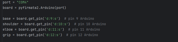
Next, let’s set up our PyFirmata environment. PyFirmata is a library that allows us to communicate with an Arduino, which we will be using to control our robot through a firmata protocol. It is a simple interface and will enable servo control directly from python rather than having to do complicated serial communication. We define where each of the servos we want to control are on the digital pins of the Arduino.
Hand Detection
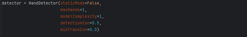
We will now initialize our hand detector. This is very simple to do as the cvzone library handles all of this.
Coordinates
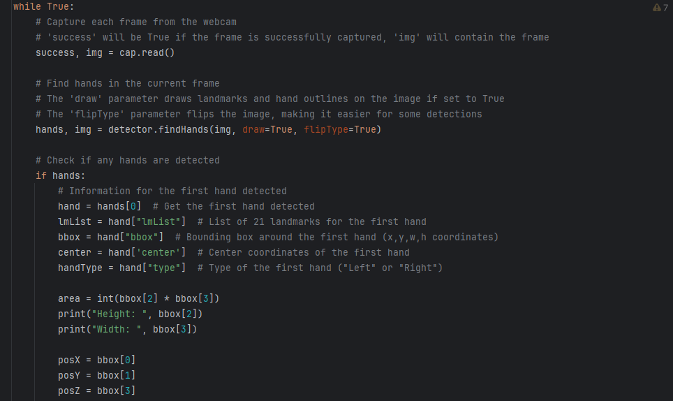
Then, we will execute our video capture and retrieve the coordinates of the hand. The code activates the OpenCV video capture and the hand detector in that video. Next, it checks if anything is detected. If so, it extracts the bounding box of the hands and where the landmarks are. Finally, we store this into our own variables to be used to input to the robot.
Robot Translation
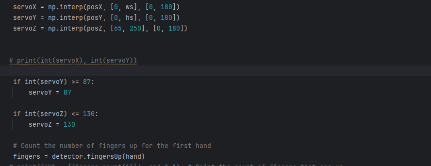
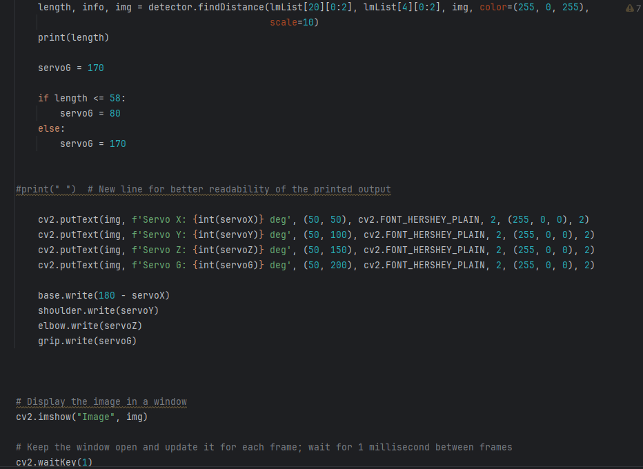
Finally, we use numpy’s interpolate function to map the coordinates that range from 0 to the screen width and height, to desired angles from 0-180 for the robotic arm. Furthermore, we also calculate the distance (Using the cvzone function) between the pinky and thumb finger (defined by lmList[20] and lmList[4]) and if they are close enough, the gripper will activate. Next, we display the angle values on the screen and send the angles to the arduino.
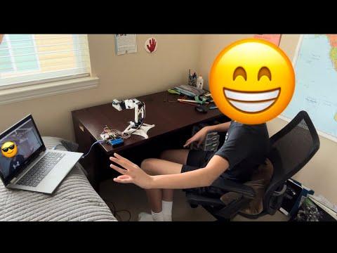
Hand Tracking Demonstration
Conclusions
The concepts of generative design and neural networks can be implemented in many mechanical and software projects. These skills are also valuable in industry and they can be the difference between a good and a great mechanical or software engineer. Generative design can be used in the optimization of almost any part. The same concepts of constraints and load cases can be applied to other software such as ANSYS and can also be utilized in FEA simulations. This instructable covered the information needed to run basic simulations and design optimization cases. In addition, the Fusion 360 generative design workspace was gone over in detail including almost all the features. Moreover, the main concepts of neural network and deep learning design in code using world-class tools were covered. This was implemented for the natural language processing and audio imaging purposes for a novel RNN-CNN voice recognition model. Furthermore, computer vision topics were discussed, diving into the details of color detection, object detection pipelines, and OpenCV fundamentals. Lastly, microcontroller serial communication was implemented to connect the developed artificial intelligence models to an actual robot and perform commands using the firmata protocol.
Way to go! You just made a state-of-the-art generative designed robotic arm using robust Fusion AI 3D Design frameworks controlled by world-class, personally developed artificial intelligence models!